Cellular Automaton Modeling of Invasive Tumor Growth: From Theoretical Foundations to Clinical Forecasting

Abstract

This comprehensive review explores the application of cellular automaton (CA) models to simulate invasive tumor growth dynamics, addressing the critical need for predictive tools in oncology. Targeting researchers, scientists, and drug development professionals, we synthesize foundational principles, methodological implementations, computational optimization strategies, and validation frameworks for CA-based tumor modeling. The article examines how these discrete computational frameworks capture emergent tumor behaviors through simple local rules, including dendritic invasion patterns, heterogeneity, and microenvironment interactions. We detail high-performance implementation techniques enabling multi-scale simulations from single cells to clinically apparent masses. Furthermore, we critically assess validation approaches integrating genomic data and clinical outcomes, positioning CA models as powerful in silico tools for probing cancer mechanisms, optimizing therapeutic strategies, and developing personalized digital twins for predictive oncology.

Understanding Tumor Invasion: Cellular Automata as Theoretical Frameworks

Fundamental Principles of Cellular Automata in Biological Systems

Cellular Automata (CA) are discrete computational models representing systems as a grid of cells, each in a finite state. The system evolves in discrete time steps according to a set of rules based on the states of neighboring cells. In biological modeling, particularly in the context of invasive tumor growth, CA provide a powerful framework for simulating complex multi-scale dynamics emerging from simple local interactions [1] [2]. They serve as in silico experiments, enabling researchers to formalize experimentally observable single-cell kinetics and observe emerging population-level dynamics without a priori knowledge of tumor behavior [1]. This approach allows for the investigation of tumor invasion and metastasis, which are crucial for both fundamental cancer research and clinical practice [2].

The core strength of CA models lies in their ability to bridge multiple spatial and temporal scales, simulating tumor growth from a single transformed cancer cell to a clinically apparent mass [1]. By incorporating a variety of microscopic-scale tumor-host interactions—including short-range mechanical interactions between tumor cells and tumor stroma, degradation of the extracellular matrix by invasive cells, and oxygen/nutrient gradient-driven cell motions—CA models can predict a rich spectrum of growth dynamics and emergent behaviors of invasive tumors [2].

Core Principles of CA Model Design

Basic Components and Structure

Every CA model is built upon four fundamental components, which must be carefully defined to realistically represent a biological system like a growing tumor.

• The Cellular Grid: The spatial foundation of the model is a lattice representing the biological environment. In tumor growth models, each grid point typically represents a physical space of approximately (10μm)², which can be occupied by a single cancer cell [1]. The grid can be structured using various geometries; for instance, a Voronoi tessellation of space into polyhedra, based on centers of spheres in a packing generated by a random sequential addition process, can model real-cell aggregates with a relatively high degree of shape isotropy [2].
• Cell States: Each cell on the grid is characterized by a specific trait vector defining its phenotype. A typical vector includes parameters such as cell cycle time (cct), proliferation potential (ρ), migration potential (μ), and rate of spontaneous death (α) [1]. Modeled tumor populations are often heterogeneous, consisting of distinct subpopulations like cancer stem cells (assumed immortal with unlimited proliferation potential) and non-stem cancer cells (with a limited number of divisions before cell death) [1].
• Neighborhood Definition: The local environment of a cell is defined by its neighborhood, which determines which other cells can influence its behavior. Common neighborhoods include the von Neumann neighborhood (four orthogonally adjacent cells) and the Moore neighborhood (all eight surrounding cells) [1]. The state of this neighborhood is critical for rules governing proliferation, migration, and quiescence; for example, cells completely surrounded by other cells in a Moore neighborhood become quiescent [1].
• Transition Rules: These are the local, often stochastic, rules that determine how a cell's state updates from one time step to the next based on its own state and the states of its neighbors. These rules formalize cellular processes such as proliferation, migration, and death. Updates are typically performed asynchronously and in random order to minimize lattice geometry effects and more accurately represent biological stochasticity [1].

Implementation for High-Performance Computing

Efficient implementation is critical for performing multi-scale Monte Carlo simulations within computationally convenient timeframes.

• Memory Architecture and Data Access: Optimizing memory access is paramount. Modern desktop PCs have layered memory: fast but small cache, slower but larger RAM, and very slow hard drives. Simulation time decreases dramatically with frequent cache misses (when required data is not in the cache). A naïve implementation using a two-dimensional array can be memory-inefficient because accessing a cell's neighbors often results in cache misses. Optimized algorithms must be designed to maximize the spatial locality of data access [1].
• Data Structures and Optimization: The choice of data structure should be guided by the expected geometry of the tumor population. For a dense, compact tumor (e.g., prostate cancer), a coded array containing information about the number of vacant spots in a cell's neighborhood can be more efficient than a simple Boolean occupancy array. Using appropriate data types (e.g., char instead of int) can reduce memory usage and improve performance by allowing more information to be stored in the cache [1].
• Random Number Generation and Ordering: Stochastic CA models require robust methods for random neighbor selection and random cell ordering. For selecting a random vacant neighboring site, an iterative method that checks neighbors in a random order until a vacancy is found is significantly faster than a naïve method that first compiles a list of all vacant spots [1]. For updating cells in a random order, using standardized library functions (e.g., the C++ STL's random_shuffle) is orders of magnitude faster than a manual approach of repeatedly selecting and erasing a random element from a vector [1].
• Dynamically Growing Domains: To simulate growth from a single cell to millions of cells without the artificial constraints of a fixed lattice boundary, the computational domain must be able to expand dynamically as the tumor population increases. This avoids the need for impractically large pre-allocated lattices, which are memory-intensive and computationally inefficient [1].

Quantitative Parameters for Tumor Growth CA

The following parameters are essential for defining the rules and states within a cellular automaton model of invasive tumor growth. They are typically derived from or calibrated against experimental data.

Table 1: Key Cellular-Level Parameters in Tumor Growth CA Models

Parameter	Description	Typical Value/Range	Biological Significance
Cell Cycle Time (cct)	The time required for a cell to complete one cycle and become eligible for division.	Scaled to discrete time steps (e.g., Δt = 1/24 day) [1]	Determines the base probability of proliferation per time step.
Proliferation Potential (ρ)	The number of divisions a non-stem cancer cell can undergo before senescence/death.	ρmax for non-stem cells; ρ=∞ for cancer stem cells [1]	Introduces cellular aging and limits the lifespan of non-stem cell lineages.
Migration Potential (μ)	The innate motility speed of a cancer cell.	Used to calculate probability of migration per time step (pm = μ×Δt) [1]	Controls the invasiveness and diffusivity of the tumor population.
Spontaneous Death Rate (α)	The probability of a cell undergoing spontaneous apoptosis in a time step.	α=0 for cancer stem cells; >0 for non-stem cells [1]	Regulates population turnover and internal tumor dynamics.
Symmetric Division Probability (ps)	The probability that a cancer stem cell division produces two stem cells.	A key parameter between 0 and 1 [1]	Governs the self-renewal versus differentiation balance of the stem cell pool.

Table 2: Model Implementation and System-Level Parameters

Parameter	Description	Considerations
Time Step (Δt)	The discrete unit of time for model advancement.	Often 1 hour (1/24 day) to balance biological accuracy and computational load [1]
Lattice Resolution	The physical space represented by a single grid point.	Typically (10μm)², approximating the size of a single cell [1]
Neighborhood Type	The definition of which grid points are considered a cell's neighbors.	Von Neumann (4 neighbors) or Moore (8 neighbors); choice affects diffusion and interaction patterns [1]
Tumor-Host Mechanics	Rules for short-range mechanical interactions with stroma/ECM.	Critical for reproducing realistic invasive patterns like dendritic branches [2]
Oxygen/Nutrient Gradient	Rules for resource-driven cell motion and proliferation.	A key driver of emergent tumor morphology and invasion [2]

Experimental Protocol: Implementing a High-Performance CA Model for Invasive Tumor Growth

This protocol details the steps for implementing a stochastic CA model to simulate invasive tumor growth, incorporating high-performance computing techniques.

Model Initialization and Setup

• Domain Configuration: Initialize a two-dimensional lattice with a size that can dynamically expand. The initial grid can be set to a modest size (e.g., 100x100), with data structures that allow seamless addition of new grid rows and columns as the tumor population grows towards the boundary [1].
• Seed the Tumor: Place a single cancer stem cell at the center of the grid. This initial cell should have its trait vector fully defined (e.g., [cct, ρ=∞, μ, α=0]) [1].
• Parameter Assignment: Define the global parameters for the simulation, including the time step (Δt = 1/24 day), probabilities for symmetric stem cell division (p_s), and the maximum proliferation potential for non-stem cells (ρ_max).

Simulation Execution Workflow

The core simulation loop advances time in discrete steps. The following workflow outlines the sequence of operations performed during each time step.

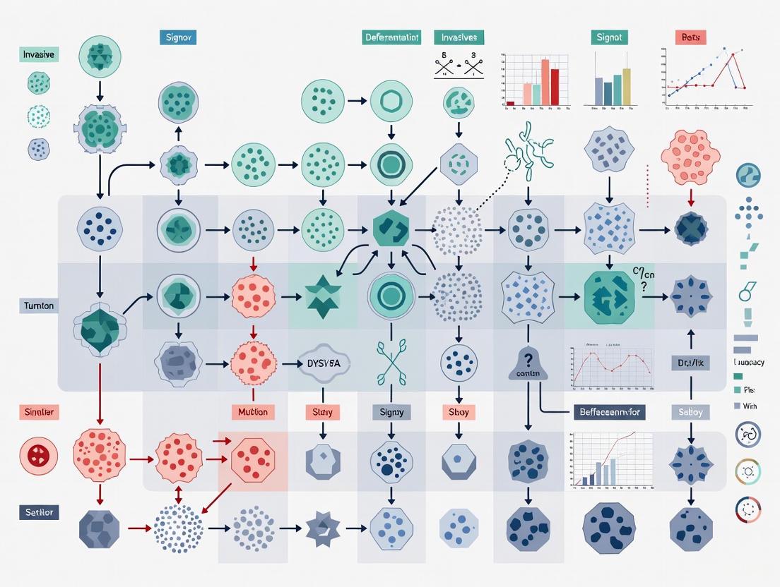
Diagram 1: CA Simulation Workflow

Key Stochastic Decision Logic

The core of the CA model lies in the stochastic decision process for each cell during its update. The following diagram details the logical sequence and probabilities involved.

Diagram 2: Stochastic Cell Update Logic

Critical Post-Simulation Analysis

• Data Collection: At predefined intervals, output simulation data for analysis. This includes the total cell count, counts of stem and non-stem cells, tumor radius (for compact masses), and the spatial coordinates of all cells for morphological analysis.
• Morphological Assessment: Quantify the emerging tumor morphology. Invasive tumors will exhibit a diffusive structure with dendritic branches, whereas non-invasive tumors will be dense and compact [1] [2]. Metrics like the fractal dimension can be used.
• Sensitivity Analysis: Perform parameter sweeps to determine which parameters (e.g., μ, p_s, α) the model is most sensitive to. This identifies critical biological parameters driving the system behavior [1].
• Statistical Validation: Run multiple simulations (≥ 100) with different random seeds for the same parameter set to obtain averaged, statistically significant results, as the model is inherently stochastic [1].

The Scientist's Toolkit: Research Reagents and Computational Solutions

Table 3: Essential Components for a Tumor Growth CA Framework

Item/Reagent	Function in the Model	Technical Notes
High-Performance Computing (HPC) Cluster	Provides the computational power for multi-scale, stochastic simulations requiring many runs.	Access to modern processors with large cache memory (e.g., Intel Xeon) significantly reduces simulation time [1].
C++ Standard Template Library (STL)	Provides optimized algorithms and data structures for efficient implementation.	Using std::random_shuffle for random cell ordering is orders of magnitude faster than naive methods [1].
Custom Cell Trait Vector	Encodes the phenotype and state of each individual cell in the simulation.	Typically implemented as a struct or object containing cct, ρ, μ, and α [1].
Dynamic Lattice Data Structure	Represents the spatially explicit grid on which cells reside and interact.	Must be dynamically growable and optimized for fast neighbor lookup and memory access [1].
Pseudorandom Number Generator (PRNG)	Drives all stochastic processes in the model (division, death, migration).	A high-quality, fast PRNG (e.g., Mersenne Twister) is essential for robust Monte Carlo simulations.
Voronoi Tessellation Generator	Creates a realistic underlying cellular structure for modeling tissue.	Used to generate polyhedral automaton cells based on random sphere packings, providing model flexibility [2].
Data Visualization Software	Analyzes and visualizes the output of simulations (tumor morphology, growth curves).	Custom scripts (e.g., in Python or MATLAB) are used to plot cell maps and analyze emergent patterns.

Cellular automaton (CA) models have emerged as powerful computational tools for simulating the complex and spatially explicit processes of invasive tumor growth. These models represent biological systems as grids of cells, each following a set of rules based on the states of neighboring cells, enabling the simulation of emergent tumor behaviors from simple local interactions. The core strength of CA modeling lies in its ability to efficiently simulate invasive tumor growth in heterogeneous host microenvironments by taking into account various microscopic-scale tumor-host interactions [3] [4]. These interactions include short-range mechanical forces between tumor cells and tumor stroma, degradation of the extracellular matrix (ECM) by invasive cells, and oxygen/nutrient gradient-driven cell motions [4]. Through these mechanisms, CA models can predict a rich spectrum of growth dynamics and emergent behaviors that correspond clinically to observed dendritic invasive patterns characterized by chains of tumor cells emanating from the primary tumor mass [3].

The transition from proliferative to invasive growth represents a critical juncture in cancer progression, often leading to metastatic dissemination and poorer patient outcomes. In vitro experiments have established that highly malignant tumors develop dendritic branches composed of tumor cells that follow each other, which massively invade into the host microenvironment [4]. CA models specifically address the formation of these invasive cell chains and their interactions with both the primary tumor mass and host microenvironment—aspects that remain poorly understood despite their clinical significance [3]. The models provide a computational framework that can integrate multiple scales of biological organization, from individual cell behaviors to tissue-level patterns, making them particularly valuable for investigating how local cellular interactions give rise to global tumor morphology and invasion dynamics.

Key Mechanisms and Emergent Behaviors in Invasive Tumors

Core Mechanisms Driving Invasive Growth

Invasive tumor progression depends on several interconnected biological mechanisms that can be effectively captured in CA models. These mechanisms operate across different spatial and temporal scales to generate the characteristic dendritic patterns observed in aggressive cancers:

• ECM Degradation and Remodeling: Invasive cells secrete proteolytic enzymes such as matrix metalloproteinases (MMPs) that degrade extracellular matrix components, creating paths of least resistance through the tumor stroma [4]. The density and distribution of ECM macromolecules significantly influence invasion patterns, with heterogeneous ECM landscapes promoting more irregular and branched invasive structures.

• Oxygen and Nutrient Gradients: Hypoxic conditions within the tumor core trigger phenotypic shifts toward invasive behaviors. Cells follow oxygen and nutrient gradients in the microenvironment, which directs their movement away from the necrotic core and toward perfused regions [4]. This chemotactic response contributes significantly to the development of dendritic invasion patterns.

• Cell-Cell and Cell-ECM Interactions: Mechanical interactions between tumor cells and between tumor cells and stroma influence invasion dynamics. CA models incorporate short-range repulsive forces and adhesion preferences that determine how cells navigate through the microenvironment [4]. Homotype attraction between tumor cells promotes the formation of chain-like structures, while heterotype interactions with stromal components can either facilitate or impede invasion.

Characteristic Emergent Behaviors

From the complex interplay of these mechanisms, several emergent behaviors arise that define invasive tumor growth:

• Dendritic Invasive Branching: The formation of chain-like structures composed of tumor cells extending from the primary tumor mass represents a hallmark emergent behavior in invasive cancers [3] [4]. These structures follow paths of least resistance through the stromal landscape and exhibit intrabranch homotype attraction, where cells maintain connectivity within invading chains.

• Nonlinear Growth Dynamics: CA models demonstrate nontrivial coupling between the growth dynamics of the primary tumor mass and invasive cells [4]. Interestingly, invasive cells can facilitate primary tumor growth in harsh microenvironments by creating channels for nutrient delivery or by remodeling the ECM to make it more permissive for expansion.

• Microenvironment-Dependent Morphology: Tumor morphology emerges dynamically from local cell-microenvironment interactions rather than being predetermined [4]. Variations in ECM density, stromal composition, and metabolic gradients yield distinct invasion patterns ranging from diffuse infiltration to highly branched dendritic structures.

Table 1: Key Emergent Behaviors in Invasive Tumor Growth and Their Clinical Correlates

Emergent Behavior	Underlying Mechanisms	Clinical/Experimental Correlates
Dendritic invasive branches	ECM degradation, homotype attraction, least-resistance pathfinding	Glioblastoma multiforme invasive patterns [4]
Metabolic niche formation	Oxygen/nutrient gradient-driven motion, hypoxic adaptation	Perinecrotic invasion zones, pseudopalisading cells
Heterogeneous growth rates	Local variations in microenvironmental resistance, resource competition	Intratumoral heterogeneity in progression rates
Therapeutic resistance emergence	Microenvironment-mediated protection, phenotypic plasticity	Recurrence after therapy, minimal residual disease

Experimental Protocols for Validating CA Model Predictions

Protocol 1: Microfluidic Single-Cell Analysis of Invasion Dynamics

Purpose: To capture single-cell behavioral data for parameterizing and validating CA models of invasive growth using microfluidic devices.

Materials and Reagents:

• Microfluidic chamber devices (e.g., passive hydrodynamic capture arrays)
• ALDEFLUOR assay kit for cancer stem cell identification
• Live-cell imaging-compatible fluorescent dyes (e.g., CellTracker)
• Appropriate cell culture media for tumor cells (varies by cell line)
• Primary tumor specimens or established tumor cell lines

Procedure:

• Device Preparation: Prime microfluidic chambers with appropriate ECM proteins (e.g., collagen I, Matrigel) to replicate tumor microenvironment conditions.
• Cell Loading: Inject single-cell suspension (100-1,000 cells/μL) into microfluidic device using passive hydrodynamic structures to capture individual cells in microchambers.
• Phenotypic Characterization: For cancer stem cell studies, perform ALDEFLUOR assay immediately after capture to determine ALDH+ status [5].
• Time-Lapse Imaging: Acquire images every 30-60 minutes for 72-120 hours using phase-contrast and fluorescence microscopy.
• Behavioral Tracking: Monitor division events, migratory behavior, and progeny phenotypes through automated or manual cell tracking.
• Data Extraction: Quantify division symmetry (symmetric vs. asymmetric), migration speed and persistence, and daughter cell fates.
• Model Parameterization: Use extracted parameters (division probabilities, migration coefficients) to inform CA model rules.

Validation Metrics:

• Percentage of quiescent cells (ALDH+ vs. ALDH- populations)
• Average number of progeny per dividing cell over observation period
• Transition probabilities between cell states (ALDH+ to ALDH-, etc.) [5]

Protocol 2: Intravital Microscopy for In Vivo Behavior Profiling

Purpose: To characterize single-cell behaviors and microenvironmental interactions in living tumors for CA model validation.

Materials and Reagents:

• Window chamber models or cranial windows for tumor imaging
• Fluorescently labeled tumor cells (e.g., GFP, RFP expressing)
• Vasculature labeling agents (e.g., dextran-conjugated fluorophores)
• Animal anesthesia and monitoring equipment
• Multiphoton or confocal intravital microscope system

Procedure:

• Tumor Implantation: Introduce fluorescently labeled tumor cells into appropriate window chamber model or orthotopic location.
• Microenvironment Labeling: Administer vascular labels or other microenvironment markers 24 hours before imaging.
• Image Acquisition: Perform multi-position, time-lapse intravital microscopy over 4-24 hour sessions with 5-15 minute intervals between time points.
• Cell Tracking: Use automated tracking software (e.g., Imaris, TrackMate) to extract single-cell trajectories and behavioral parameters.
• Microenvironment Mapping: Correlate cell behaviors with local microenvironmental features (vasculature, immune cells, ECM density).
• Behavioral Classification: Apply computational tools (e.g., BEHAV3D Tumor Profiler) to classify cells based on morphodynamic profiles [6].
• Model Comparison: Compare observed behavioral distributions and microenvironmental associations with CA model predictions.

Validation Metrics:

• Proportion of motile vs. stationary cells
• Migration speed and persistence parameters
• Association between specific TME features and cell behaviors
• Spatial distribution of behavioral subtypes within tumors [6]

Computational Implementation of CA Models for Invasive Growth

Model Framework and Implementation

CA models for invasive tumor growth typically employ a Voronoi tessellation framework, which provides a more biologically realistic representation of cellular packing compared to regular grids. The model space is partitioned into polyhedral automaton cells based on centers of spheres in a packing generated by a random sequential addition process [4]. Each automaton cell can represent either a single tumor cell or a region of tumor stroma, with linear sizes approximating 10-20μm to match biological scales.

The simulation domain typically spans several millimeters, containing up to 250,000 automaton cells in 2D implementations [4]. Each ECM-associated automaton cell is assigned a specific density value (ρECM) representing the density of ECM macromolecules within that region. Tumor cells can only occupy an ECM-associated automaton cell if the density falls below a critical threshold, either through natural ECM heterogeneity or active degradation by invasive cells.

Table 2: Key Parameters in CA Models of Invasive Tumor Growth

Parameter Category	Specific Parameters	Biological Significance	Typical Values/Ranges
Cell Behavioral Parameters	Proliferation probability	Controls expansion rate of tumor population	0.1-0.8 per cell cycle
	Migration probability	Determines invasive potential	0.05-0.5 per time step
	ECM degradation capacity	Ability to remodel microenvironment	0-1.0 units per time step
Microenvironmental Parameters	ECM density distribution	Determines structural resistance to invasion	0-1.0 (normalized)
	Oxygen/nutrient gradients	Drives directed migration	0-100% of vascular source
	Stromal cell density	Influences cell-cell interactions	0-80% of volume
Transition Rules	Homotype attraction	Promotes chain formation	Binary or weighted
	Heterotype adhesion	Controls stromal interactions	0-1.0 (adhesion strength)
	Phenotypic switching	Models plasticity in response to cues	0.001-0.1 probability

Rule Implementation and Model Execution

The CA model progresses through discrete time steps, with each tumor cell evaluating possible actions based on its current state and local microenvironment:

• Proliferation Check: Cells evaluate proliferation probability based on local nutrient availability and cell-cycle status.
• Migration Assessment: Motile cells determine direction and probability of movement based on ECM density, gradient sensing, and contact guidance.
• ECM Interaction: Cells attempt to degrade local ECM if density exceeds invasion thresholds.
• State Updates: All cell states and microenvironment parameters are updated synchronously after all cells have executed their actions.

The model incorporates both deterministic rules (e.g., nutrient consumption) and stochastic elements (e.g., probability of division) to capture the inherently probabilistic nature of cellular decision-making. This combination enables the emergence of realistic tumor behaviors from relatively simple local rules.

Diagram 1: Framework of emergent behaviors in CA tumor models showing how local rules generate global patterns.

Integration with Experimental Data and Model Validation

Parameter Estimation from Experimental Systems

Effective parameterization of CA models requires quantitative data from experimental systems that capture specific aspects of tumor invasion:

Cancer Stem Cell Dynamics: Microfluidic single-cell culture data reveals distinct behavioral differences between ALDH+ and ALDH- cells that must be incorporated into CA models. ALDH+ cells demonstrate higher proliferative capacity (4.4 vs. 2.2 progeny per dividing cell in SKOV3 lines) and lower quiescence rates (12% vs. 35% in SKOV3) compared to ALDH- cells [5]. These differential behaviors significantly impact long-term tumor growth dynamics and invasion patterns.

Single-Cell Migration Profiling: Intravital microscopy coupled with computational tools like BEHAV3D-TP enables quantification of heterogeneous migratory behaviors in the native tumor microenvironment [6]. This approach can identify distinct migration subtypes (random, directional, confined) and correlate them with local microenvironmental features such as vasculature proximity or immune cell densities.

ECM Heterogeneity Mapping: Second harmonic generation imaging and other ECM characterization techniques provide spatial maps of collagen density and organization that can directly inform the initial conditions of CA model simulations. These structural parameters significantly influence the paths taken by invasive cells and the resulting dendritic patterns.

Multi-scale Validation Approaches

Validating CA model predictions requires comparison with experimental data across multiple spatial and temporal scales:

• Cellular Scale: Compare simulated and observed proportions of migratory vs. proliferative cells, division symmetries, and phenotypic transitions.
• Multicellular Scale: Evaluate similarity between simulated and experimentally observed invasive chain structures, including branch length distributions and connectivity patterns.
• Tissue Scale: Assess correspondence between simulated and actual tumor morphologies, invasion fronts, and spatial relationships with host tissue structures.

Diagram 2: Workflow for parameterizing and validating CA tumor models with experimental data.

Application Notes for Drug Development

Targeting Emergent Invasive Behaviors

CA models offer unique opportunities for simulating therapeutic interventions and identifying potential vulnerabilities in invasive tumor systems:

ECM-Modifying Therapies: Simulations can test how alterations in ECM density or composition affect invasive patterns. Models predict that moderate ECM disruption can paradoxically enhance invasion by creating microtracks for cell migration, while more substantial ablation may constrain invasive outgrowth [4]. These non-intuitive outcomes highlight the value of CA models in optimizing therapeutic ECM targeting strategies.

Metabolic Intervention Strategies: By incorporating oxygen and nutrient gradients, CA models can simulate how metabolic interventions alter invasion dynamics. Simulations suggest that targeting hypoxic adaptation mechanisms may preferentially disrupt chain formation in dendritic branches, potentially suppressing metastatic dissemination.

Phenotypic Switching Inhibitors: CA models incorporating cancer stem cell plasticity can test strategies that limit transitions between proliferative and invasive states. Simulation results indicate that even modest reductions in phenotypic switching probabilities can significantly delay the emergence of invasive branches without substantially affecting primary tumor growth [5].

Protocol 3: In Silico Therapeutic Screening Using CA Models

Purpose: To utilize CA models for predicting therapeutic responses and identifying potential resistance mechanisms in invasive tumors.

Computational Requirements:

• High-performance computing cluster or multi-core workstation
• Custom CA simulation software (typically MATLAB, Python, or C++)
• Parameter optimization algorithms
• Data visualization and analysis pipelines

Procedure:

• Baseline Calibration: Parameterize CA model using patient-derived or cell line-specific data to establish untreated growth and invasion dynamics.
• Therapeutic Integration: Implement therapy-specific rules into the CA framework:
  • Cytotoxic agents: Increase probability of cell death based on proliferation status
  • Anti-invasive agents: Modify migration probabilities or ECM degradation capacities
  • Microenvironment-targeting: Alter ECM density distributions or nutrient gradients
• Dose-Response Simulation: Execute multiple simulation runs across a range of therapeutic intensities and timing schedules.
• Response Quantification: Extract metrics including:
  • Primary tumor volume reduction
  • Invasive branch length and complexity
  • Cancer stem cell fraction dynamics
  • Spatial patterns of residual disease
• Resistance Analysis: Identify potential escape mechanisms through sensitivity analysis of model parameters.
• Combination Screening: Simulate combination therapies to identify synergistic effects on invasion suppression.

Output Analysis:

• Time to recurrence metrics under different treatment scenarios
• Spatial distribution of treatment-resistant niches
• Optimal therapeutic sequencing to prevent invasion
• Biomarker predictions for patient stratification

Table 3: Essential Research Reagent Solutions for Investigating Invasive Tumor Behaviors

Resource Category	Specific Tools/Reagents	Research Application	Key Features
Computational Tools	BEHAV3D Tumor Profiler [6]	Analysis of single-cell behaviors in IVM data	Google Colab integration, no coding requirement
	Voronoi-based CA framework [4]	Simulation of invasive growth patterns	Biologically realistic cell packing, ECM integration
	Microfluidic device analysis [5]	Single-cell tracking and fate mapping	ALDH+ cell identification, division symmetry analysis
Experimental Models	Window chamber models [6]	Intravital imaging of tumor dynamics	Real-time behavior in native microenvironment
	3D organotypic cultures	ECM invasion assays	Controlled microenvironmental conditions
	Patient-derived xenografts	Therapeutic response validation	Maintains tumor heterogeneity and microenvironment
Analytical Reagents	ALDEFLUOR assay [5]	Cancer stem cell identification	Live-cell sorting and tracking capability
	ECM fluorescent conjugates	Matrix remodeling visualization	Second harmonic generation compatibility
	Photoactivatable fluorescent proteins	Cell lineage tracing	Spatiotemporal fate mapping

Cellular automaton modeling represents a powerful approach for understanding and predicting emergent behaviors in invasive tumor growth. By integrating multiple scales of biological organization—from molecular cues to cellular decision-making to tissue-level patterns—CA models provide unique insights into the fundamental principles governing dendritic invasion and metastatic progression. The protocols and applications outlined in this document provide researchers with practical frameworks for employing these models in both basic research and therapeutic development contexts.

Future advancements in CA modeling will likely focus on increasing biological fidelity through incorporation of omics data, enhancing computational efficiency for high-throughput therapeutic screening, and improving integration with clinical imaging data for personalized prediction. As these models continue to evolve, they hold increasing promise as in silico platforms for understanding cancer complexity and optimizing therapeutic strategies against invasive cancers.

Modeling Tumor-Host Microenvironment Interactions

The emergence of invasive and metastatic behavior in malignant tumors often leads to fatal outcomes for patients [4] [7]. These complex processes result from multifaceted tumor-host interactions and inter-cellular dynamics that remain poorly understood. Cellular automaton (CA) models have emerged as powerful computational tools to investigate microenvironment-enhanced invasive growth of avascular solid tumors, enabling researchers to simulate individual cell behaviors and their collective outcomes [4] [8] [7].

Unlike continuum models that treat tumors as homogeneous masses, CA models capture discrete cell-scale interactions, including extracellular matrix (ECM) degradation, nutrient-driven cell migration, pressure accumulation from microenvironment deformation, and cell-cell adhesion effects [7]. This granular approach allows researchers to reproduce hallmark invasive behaviors observed experimentally, such as elongated invasion branches characterized by homotype attraction and least-resistance paths [4]. The integration of clinical data with these in silico models provides a promising pathway toward predicting neoplastic progression and developing individualized treatment strategies [4] [8].

Biological Foundation of Tumor Microenvironment Interactions

The tumor microenvironment represents a complex ecosystem where malignant cells interact with diverse host elements, including stromal cells, immune components, and the extracellular matrix [4] [9]. The ECM provides both mechanical support and biochemical signaling cues, with its composition and density significantly influencing tumor progression [4] [10]. In highly malignant tumors such as glioblastoma multiforme, experimental observations reveal dendritic invasive branches composed of chains of tumor cells emanating from the primary tumor mass [4].

Key Biological Processes in Tumor Invasion

Tumor invasion involves a multistep process including homotype detachment, enzymatic matrix degradation, integrin-mediated heterotype adhesion, and active, directed motility [4]. Malignant cells exhibit remarkable adaptability, modifying their local microenvironment through ECM degradation while responding to chemotactic gradients [4] [7]. Myeloid-derived suppressor cells (MDSCs) play a crucial role in shaping the pre-metastatic niche by promoting immunosuppression and angiogenesis [9] [11]. These cells interact with vascular endothelial cells, immune effectors, and matrix-metalloproteinases (MMPs) to create a permissive environment for tumor progression [9].

Computational Framework: Cellular Automaton Modeling

Model Foundation and Structure

The cellular automaton model for invasive tumor growth employs a Voronoi tessellation approach, creating polyhedral automaton cells based on centers of spheres in a packing generated by random sequential addition [4]. This geometrical framework provides a flexible model for real-cell aggregates with relatively high shape isotropy, minimizing undesired growth bias compared to ordered tessellations based on regular lattices [4]. Each automaton cell typically represents either a single tumor cell or a region of tumor stroma, with a linear size of approximately 10μm, enabling simulations of domains containing millions of cells [4].

The model incorporates several key microscopic-scale tumor-host interactions:

• ECM degradation by malignant cells
• Nutrient-driven cell migration along oxygen/nutrient gradients
• Pressure accumulation due to microenvironment deformation by growing tumor
• Cell-cell adhesion effects on collective tumor behavior [7]

Mathematical Formulation

The CA model updates cell states based on rules incorporating both local interactions and microenvironmental factors. The mathematical framework includes mechanical interactions between tumor cells and tumor stroma, ECM degradation dynamics, and nutrient gradient-driven cell motility [4] [7]. Each ECM-associated automaton cell is assigned a specific density value ρECM, representing the density of ECM macromolecules within that cell [4]. A tumor cell can only occupy an ECM-associated automaton cell if ρECM < ρcritical, indicating that the ECM has been sufficiently degraded or displaced by proliferating tumor cells [4].

The model successfully reproduces emergent invasive behaviors, including the observation that invasive cells can facilitate primary tumor growth in harsh microenvironments—a non-trivial coupling effect between primary and invasive cell populations [4] [8].

Experimental Protocols and Methodologies

Protocol 1: Implementing the Core CA Model for Tumor Growth

Purpose: To establish the foundational CA framework for simulating invasive tumor growth in heterogeneous microenvironments.

Materials and Computational Setup:

• Simulation domain of approximately 5mm linear size
• Voronoi tessellation with approximately 250,000 automaton cells
• Variable ECM density distribution (ρECM) across automaton cells
• Defined nutrient/oxygen gradient parameters

Procedure:

• Initialize Voronoi Grid: Generate Voronoi tessellation based on random sequential addition of sphere centers until saturation [4]
• Define Microenvironment: Assign heterogeneous ECM density values to automaton cells using predetermined distribution patterns
• Seed Tumor Cells: Place initial tumor cells at designated locations within the simulation domain
• Set Nutrient Gradients: Establish initial oxygen/nutrient concentration fields
• Implement Update Rules: Apply CA rules for each time step, including:
  • Cell proliferation probability based on local nutrient levels
  • Cell migration along nutrient gradients
  • ECM degradation when ρECM < ρcritical
  • Pressure accumulation and its effect on tumor-host interface stability
  • Cell-cell adhesion effects [4] [7]
• Execute Simulation: Run for predetermined number of time steps or until reaching specified tumor size
• Data Collection: Record tumor morphology, invasive branch characteristics, and cell distribution patterns

Validation: Compare simulated patterns with experimentally observed dendritic invasive branches characterized by intrabranch homotype attraction and least-resistance paths [4]

Protocol 2: Investigating ECM Properties and Cell-Adhesion Effects

Purpose: To systematically analyze how ECM rigidity and cell-cell adhesion strength collectively influence tumor invasion patterns.

Materials and Setup:

• Parameter sweep of ECM density (rigidity) values
• Range of cell-cell adhesion strength parameters
• Fixed nutrient gradient conditions
• Consistent initial tumor seeding

Procedure:

• Parameter Matrix Setup: Create comprehensive parameter matrix combining ECM density and cell-adhesion values
• Simulation Series: Execute full CA simulations for each parameter combination
• Invasion Metrics: Quantify invasion extent using:
  • Number of invasive branches
  • Branch length distribution
  • Surface roughness of primary tumor mass
• Phase Diagram Construction: Map parameter combinations to resulting invasion phenotypes [7]
• Transition Boundary Identification: Determine critical parameter values marking non-invasive to invasive transition

Analysis: The protocol enables construction of a "phase diagram" summarizing tumor invasive behavior dependency on ECM rigidity and cell-cell adhesion strength, revealing clear transitions from non-invasive to invasive phenotypes with increasing ECM rigidity and/or decreasing cell-cell adhesion [7]

Protocol 3: Hybrid CA-PDE Modeling of Tumor-Immune Interactions

Purpose: To incorporate immune system components into the tumor growth model using a hybrid cellular automaton-partial differential equation approach.

Materials and Setup:

• CA framework for tumor and immune cell populations
• Reaction-diffusion PDEs for chemical species (nutrients, cytokines)
• Immune cell parameters (migration, recognition, killing efficacy)

Procedure:

• Extended CA Setup: Implement additional cell states for immune populations (e.g., effector cells, MDSCs)
• PDE Component: Establish reaction-diffusion equations for chemical fields:
  • Nutrient concentrations
  • Chemoattractant gradients
  • Immune signaling molecules [12]
• Coupling Mechanism: Define interfaces between discrete CA cells and continuous PDE fields
• Immune Cell Rules: Implement behavioral rules for immune components:
  • Chemotactic migration along cytokine gradients
  • Tumor cell recognition and elimination probabilities
  • Immune suppression mechanisms [9] [12]
• Integrated Simulation: Execute coupled CA-PDE model with appropriate time stepping
• Outcome Assessment: Evaluate tumor-immune dynamics including:
  • Immune infiltration patterns
  • Tumor escape mechanisms
  • Oscillatory growth behaviors [12]

Applications: This protocol enables investigation of immunotherapeutic strategies and analysis of spatial patterns of immune cell infiltration in relation to collagen alignment and other ECM characteristics [13]

Key Findings and Quantitative Data

Emergent Tumor Invasion Behaviors

The CA model robustly reproduces several hallmark invasion patterns observed in experimental studies:

• Dendritic Invasive Branches: Formation of chain-like tumor cell structures emanating from primary mass [4] [8]
• Least-Resistance Path Selection: Invasive cells follow paths of minimal mechanical resistance [4] [7]
• Intrabranch Homotype Attraction: Maintaining connectivity within invasive branches [4]
• Surface Roughness Development: In high-pressure confined environments [7]
• Invasive-Facilitated Growth: Invasive cells can enhance primary tumor growth in harsh microenvironments [4]

Parameter Dependencies and Phase Transitions

Comprehensive simulations reveal how tumor invasion patterns depend critically on microenvironmental parameters:

Table 1: Tumor Invasion Dependencies on Microenvironment Parameters

Parameter	Effect on Invasion	Experimental Correlation
High ECM density/rigidity	Promotes invasive behavior	Correlates with malignant progression [7]
Weak cell-cell adhesion	Enhances cell dispersal and invasion	Associated with epithelial-mesenchymal transition [7]
Steep nutrient gradients	Directs invasive branch growth	Observed in hypoxic tumor regions [4]
High mechanical pressure	Increases surface roughness	Found in confined tumor environments [7]
Aligned collagen fibers	Facilitates directed invasion	Correlates with poor prognosis in squamous cell carcinomas [13]

Table 2: Classification of Tumor Growth Morphotypes in CA Simulations

Morphotype	Characteristic Features	Governed By
Spherical growth	Smooth, confined tumor boundary	High cell-cell adhesion, low ECM density [12] [7]
Papillary growth	Branching projections	Intermediate adhesion and ECM density [12]
Dendritic invasion	Elongated chains of tumor cells	Low adhesion, high ECM density, nutrient gradients [4]
Oscillatory growth	Phases of growth and regression	Strong immune interaction with intermediate killing efficacy [12]
Immune infiltration	Mixed tumor-immune cell distribution	High immune chemotaxis and recognition [12] [13]

The phase diagram constructed from simulation data demonstrates a clear transition from non-invasive to invasive behaviors with increasing ECM rigidity and/or decreasing cell-cell adhesion strength [7]. This quantitative relationship provides testable predictions for experimental investigation of invasion thresholds.

The Scientist's Toolkit: Research Reagent Solutions

Table 3: Essential Research Reagents and Computational Tools for Tumor Microenvironment Modeling

Reagent/Tool	Function/Application	Example Use in Studies
Voronoi tessellation	Underlying cellular structure for CA	Provides geometrical framework for cell interactions [4]
ECM density mapping	Represents heterogeneous host microenvironment	Models variation in tissue mechanical properties [4] [7]
Nutrient gradient field	Drives chemotactic cell migration	Simulates oxygen/nutrient distribution in tumor tissue [4] [12]
Matrix metalloproteinases (MMPs)	ECM degradation and remodeling	Facilitates tumor cell invasion through matrix barriers [9] [11]
Myeloid-derived suppressor cells (MDSCs)	Immune suppression in pre-metastatic niche	Creates permissive environment for metastasis [9] [11]
Hybrid CA-PDE framework	Couples discrete cells with continuum fields	Models tumor-immune interactions with chemical signaling [12]
Lenia extended CA	Continuous space-time cellular automata	Captures complex tumor-immune-ECM dynamics [13]
3D spheroid cultures	Experimental validation of model predictions	Provides physiological relevant invasion assays [10]

Computational Visualizations

Tumor Invasion Mechanisms and Microenvironment Interactions

Diagram 1: Tumor Invasion Mechanism Network. This visualization illustrates how microenvironmental factors influence cellular processes to generate specific tumor invasion patterns, as captured by cellular automaton models.

Hybrid CA-PDE Modeling Workflow

Diagram 2: Hybrid CA-PDE Modeling Workflow. This diagram outlines the integrated computational framework combining discrete cellular automaton rules with continuous partial differential equations for simulating tumor-microenvironment interactions.

Invasion Phase Transition Diagram

Diagram 3: Tumor Invasion Phase Transition. This visualization represents the transition from non-invasive to invasive tumor behaviors based on ECM density and cell-cell adhesion parameters, as predicted by comprehensive CA simulations [7].

Cellular automaton modeling provides a powerful computational framework for investigating the complex dynamics of tumor-host microenvironment interactions. By incorporating discrete cell-scale interactions and microenvironmental factors, CA models successfully reproduce hallmark invasive behaviors and reveal how parameter variations drive transitions between non-invasive and invasive phenotypes. The protocols and methodologies outlined in this application note equip researchers with tools to simulate, analyze, and predict tumor progression patterns, potentially contributing to improved therapeutic strategies and personalized treatment approaches in clinical oncology.

This document provides application notes and detailed experimental protocols for quantifying the four key cellular processes—proliferation, migration, apoptosis, and quiescence—in the context of cancer research. These protocols are designed to generate quantitative data essential for parameterizing and validating cellular automaton models of invasive tumor growth. Such agent-based computational models simulate tumor dynamics by defining rules for individual cell behaviors, including division, movement, death, or entry into a dormant state [14]. The data obtained from these methods allows for the accurate calibration of in silico models, enabling the virtualization of different tumor growth scenarios and the testing of therapeutic hypotheses [14] [15].

The following tables consolidate key quantitative indices and parameters for the core cellular processes, as reported in experimental and clinical studies.

Table 1: Experimentally Measured Proliferation and Apoptosis Indices in Human Retinoblastoma Tumors.

Process	Quantitative Index	Mean Value ± SD	Measurement Method	Clinical/Experimental Correlation
Proliferation	Proliferative Index (PI)	37.63 ± 11.12	Ki67 immunohistochemical staining [16]	Directly proportional to tumor dimensions (P = .001) [16]
Apoptosis	Apoptotic Index (AI)	2.67 ± 1.18	TUNEL assay [16]	AI > 2.4% associated with lower PI and no observed metastasis (P = .014) [16]

Table 2: Phenotypic Ranges and Associations from Breast Cancer Studies.

Cellular Process	Experimental Context	Measured Value/Range	Association with Disease Aggressiveness
Proliferation	Breast cancer cell lines [17]	Varying doubling times across 46 cell lines	Increases with tumor stage and grade [17]
Migration	Breast cancer cell lines [17]	Varying mean migration speeds across 43 cell lines	More strongly associated with patient survival than proliferation [17]
Quiescence	Tumor Dormancy [14]	Modelled as a reversible state in cellular automata	Associated with tumor dormancy periods and therapy resistance [14]

Detailed Experimental Protocols

Protocol: Measuring Proliferation Using Direct Cell Counting and Live-Cell Imaging

This protocol details two methods for quantifying proliferation rates: endpoint direct counting and continuous live-cell imaging [15].

Materials and Reagents

• Cell culture of interest (e.g., cancer cell lines)
• Complete cell culture medium
• Trypsin or Accutase solution for dissociation
• Trypan blue solution or other viability dye
• Hemacytometer or automated cell counter (e.g., Countess, NucleoCounter)
• Tissue culture-treated plates or flasks
• Live-cell imaging system (e.g., fluorescent microscope with environmental chamber)
• Optional: Fluorescent nuclear stains (e.g., Hoechst dyes), lipophilic membrane dyes, or stable fluorescent protein constructs (e.g., GFP) [15]

Procedure: Endpoint Direct Cell Counting

• Seed cells at a known, low density in a multi-well plate or flask. Include sufficient replicates.
• Incubate cells under standard conditions for a defined period.
• Dissociate adherent cells by washing with PBS and incubating with trypsin/Accutase until cells detach.
• Neutralize the dissociation agent with complete medium and collect the cell suspension.
• Mix cell suspension with trypan blue solution and count viable cells using a hemacytometer or automated cell counter.
• Calculate proliferation rate by comparing cell counts at the end of the experiment to the seeding density. For dynamic estimates, repeat counts at multiple time points and fit the data to an exponential or logistic growth model [15].

Procedure: Continuous Live-Cell Imaging

• Seed cells in a plate compatible with live-cell imaging.
• Optional: Label cells with a fluorescent marker (e.g., Hoechst for nuclei, stable GFP expression) to facilitate automated segmentation and tracking [15].
• Place the plate in a live-cell imaging system maintaining 37°C and 5% CO₂.
• Acquire images at regular intervals (e.g., every 15-30 minutes) over 24-72 hours.
• Analyze images using cell segmentation and tracking software to generate continuous cell count data over time.

Protocol: Measuring Migration Using Live-Cell Imaging and Tracking

This protocol describes a method to quantify random cell migration, a key phenotype in cancer invasion [17].

Materials and Reagents

• Cell culture of interest
• Complete cell culture medium
• Live-cell imaging system
• Tissue culture-treated plates, preferably with low-reflection glass bottoms

Procedure

• Seed cells at a low density to ensure individual cells can be tracked without collisions.
• Allow cells to adhere and stabilize under standard conditions.
• Place the plate in the live-cell imaging system maintaining 37°C and 5% CO₂.
• Acquire phase-contrast or fluorescent images at frequent intervals (e.g., every 5-10 minutes) over 12-24 hours.
• Track cell movements using automated cell tracking software (e.g., TrackMate in ImageJ, or commercial solutions).
• Quantify migration by calculating the mean speed (total path length divided by time) or the persistence of individual cells [17].

Protocol: Measuring Apoptosis Using the TUNEL Assay

This protocol outlines the TUNEL method for detecting apoptotic cells in situ via labeling of DNA fragmentation [16].

Materials and Reagents

• Tissue sections or cell pellets fixed in 4% paraformaldehyde
• Proteinase K solution
• Terminal deoxynucleotidyl transferase (TdT) enzyme
• Labeled nucleotides (e.g., fluorescein-dUTP)
• Blocking solution (e.g., BSA)
• Counterstain (e.g., DAPI for nuclei)
• Fluorescence microscope

Procedure

• Deparaffinize and rehydrate tissue sections if using paraffin-embedded samples.
• Treat with Proteinase K to permeabilize the tissue and expose DNA.
• Incubate with TdT enzyme and labeled dUTP to label the 3'-ends of fragmented DNA.
• Wash to stop the reaction and remove unincorporated nucleotides.
• Apply a blocking solution to reduce non-specific background.
• Mount with an anti-fade medium containing a nuclear counterstain like DAPI.
• Visualize and count under a fluorescence microscope. The Apoptotic Index (AI) is calculated as the percentage of TUNEL-positive cells among the total number of cells counted [16].

Signaling Pathways and Experimental Workflows

The following diagrams, generated with Graphviz DOT language, illustrate the core signaling pathways influencing these cellular processes and the workflows for the key experimental protocols.

Signaling Pathways in Key Cellular Processes

Cellular Process Signaling Pathways

Experimental Protocol Workflow

Experimental Protocol Workflow

The Scientist's Toolkit: Research Reagent Solutions

Table 3: Essential Reagents and Materials for Cellular Process Analysis.

Reagent/Material	Function/Application	Example Use Case
Ki-67 Antibody [16]	Immunohistochemical detection of proliferating cells.	Quantifying the Proliferative Index (PI) in tumor sections.
TUNEL Assay Kit [16]	In situ labeling of DNA strand breaks for apoptosis detection.	Calculating the Apoptotic Index (AI) in fixed tissue or cells.
Bromodeoxyuridine (BrdU) [15]	Nucleoside analog incorporated during DNA synthesis for proliferation tracking.	Label dilution assays to measure division history in cell populations.
Fluorescent Nuclear Stains (Hoechst) [15]	Labeling nuclei for live-cell imaging and automated cell counting.	Segmenting and tracking cells in proliferation and migration assays.
Stable Fluorescent Proteins (GFP, RFP) [15]	Genetically encoded labels for long-term cell tracking.	Lineage tracing and monitoring co-cultured cell populations over time.
Metabolic Assay Kits (MTT, MTS, Resazurin) [15]	Measuring metabolic activity as a proxy for cell viability/proliferation.	High-throughput screening of drug effects on cell growth.
Cell Dissociation Agents (Trypsin, Accutase) [15]	Detaching adherent cells for endpoint counting and subculturing.	Harvesting cells for direct cell count proliferation measurements.

The hierarchical organization of tumors, comprising a subpopulation of Cancer Stem Cells (CSCs) and a larger population of non-stem cancer cells (NSCCs), is a critical driver of tumor initiation, progression, metastasis, and therapeutic resistance [18]. Integrating this cellular heterogeneity into cellular automaton (CA) models of invasive tumor growth is essential for developing biologically realistic in silico platforms capable of predicting neoplastic progression and testing therapeutic strategies [1] [2].

CSCs exhibit capacities for self-renewal, unlimited proliferation, and the generation of heterogeneous tumor cell lineages through asymmetric division. In contrast, NSCCs possess limited proliferation potential and will eventually undergo cell death after a finite number of divisions [1]. This functional distinction is a fundamental source of intratumoral heterogeneity and must be explicitly encoded into the rules governing cell behavior within a CA framework to accurately simulate long-term tumor dynamics and relapse following treatment [18].

Quantitative Definitions for CA Modeling

Table 1: Defining Core Cell Population Parameters for CA Models

Parameter	Cancer Stem Cell (CSC)	Non-Stem Cancer Cell (NSCC)
Proliferation Potential (ρ)	Unlimited (ρ = ∞) [1]	Limited (ρ = ρmax), decrements with each division [1]
Spontaneous Death Rate (α)	Typically α = 0 [1]	α > 0 [1]
Division Mode	Symmetric: Two CSCs (Probability ps)Asymmetric: One CSC + one NSCC (Probability 1-ps) [1]	Symmetric: Two NSCCs [1]
Key Molecular Markers	CD44, CD133, KLF4, SOX2, OCT4, C-MYC, BMI1 [18] [19] [20]	Varies by differentiated cell type
Primary Function in Model	Tumor initiation, long-term propagation, and regeneration [18] [20]	Contribution to tumor bulk and volume [1]

Table 2: Key Signaling Pathways and Their Roles in CSC Regulation

Pathway/Process	Core Components	Functional Impact on CSCs	Therapeutic Implication
Stemness Pluripotency	KLF4, SOX2, OCT4, C-MYC, BMI1 [19] [20]	Maintains self-renewal and undifferentiated state [19]	Co-targeting BMI1 and MYC prevents CSC regeneration and relapse [20]
Epithelial-Mesenchymal Transition (EMT)	TWIST1, SNAIL1, ZEB1, Vimentin, N-cadherin (Upregulated); E-cadherin (Downregulated) [19]	Enhances invasion, migration, and dissemination [19]	Targeting EMT regulators may suppress metastasis
Drug Resistance	ABCB1, ABCC1 (ABC Transporters) [19]	Mediates efflux of chemotherapeutic drugs (e.g., 5-FU) [19]	ABC transporter inhibition can re-sensitize tumors
Inflammatory Reprogramming	NF-κB, IL-6, MYC [20]	Drives the reversion of NSCCs to CSCs post-therapy [20]	NF-κB/IL-6/MYC axis blockade prevents adaptive resistance

Experimental Protocols for CSC Validation and Model Parameterization

To ensure a CA model is grounded in experimental biology, the following protocols provide methodologies for obtaining and validating CSC populations, the data from which can be used to parameterize model rules.

Protocol 1: Enriching CSCs via Chronic Chemotherapy Exposure

This protocol enriches for therapy-resistant CSCs by mimicking clinical adaptation through prolonged exposure to sub-lethal doses of chemotherapeutic agents, such as 5-Fluorouracil (5-FU) [19].

Research Reagent Solutions:

• 5-Fluorouracil (5-FU): A standard chemotherapeutic agent used for selection pressure to enrich for drug-resistant CSC populations [19].
• MTT Assay Reagent: (3-(4,5-Dimethylthiazol-2-yl)-2,5-diphenyltetrazolium bromide) used for cytotoxicity assays to determine cell viability and IC50 values [19].
• DMEM/F12 Serum-Free Medium: A base medium for spheroid culture, supplemented with growth factors to select for stem-like cells [19].
• Growth Factor Supplements (EGF & bFGF): Epidermal Growth Factor and basic Fibroblast Growth Factor are essential components of serum-free medium to support CSC survival and proliferation in spheroid assays [19].
• B27 Supplement: A serum-free supplement providing hormones, proteins, and other factors necessary for CSC growth in defined, non-differentiating conditions [19].
• Poly-HEMA: (Poly(2-hydroxyethyl methacrylate)) used to coat culture dishes to prevent cell attachment, thereby forcing cells to grow in suspension and form spheroids [19].
• CFSE Cell Division Tracker Kit: (Carboxyfluorescein succinimidyl ester) used to monitor and track cell proliferation rates [19].

Procedure:

• IC50 Determination: Seed cells (e.g., HT-29 or Caco2 colorectal cancer lines) at 10,000 cells/well in a 96-well plate. After 24 hours, expose cells to a serial dilution of 5-FU (e.g., from 6.25 ng/mL to 25600 ng/mL) for 48 hours. Assess cell viability using the MTT assay per manufacturer's instructions to calculate the IC50 value [19].
• Chronic Drug Selection: Culture 4 x 10^6 cells in T25 flasks. Initiate selection with a 5-FU concentration equivalent to 25% of the IC50.
• Cyclic Exposure: Subject cells to a repeating 7-day cycle:
  • Day 1-4: Culture cells in medium containing the current 5-FU concentration.
  • Day 5: Replace with drug-free medium for a 1-day recovery.
  • Day 6: Trypsinize cells.
  • Day 7: Culture in drug-free medium for a second recovery day.
• Dose Escalation: After each 7-day cycle, double the 5-FU concentration for the next cycle. Repeat for 7 cycles, resulting in a final exposure concentration 128 times the initial starting dose [19].
• Validation: Characterize the resulting resistant population using the assays outlined in Protocol 3.

Protocol 2: Enriching CSCs via Spheroid Formation

This method exploits the ability of CSCs to survive and proliferate under non-adherent, serum-free conditions, forming 3D structures called spheroids [19].

Procedure:

• Cell Preparation: Detach parental cells using 0.05% trypsin/EDTA. Neutralize trypsin, wash cells twice with PBS, and resuspend in pre-warmed, serum-free DMEM/F12 medium. This medium must be supplemented with 20 ng/mL EGF, 10 ng/mL bFGF, 2% B27 supplement, 1% non-essential amino acids, and 2 mM L-glutamine [19].
• Hanging Drop Method (for initial formation): For cell lines like HT-29, create a suspension of 5,000-10,000 cells in 25 µL of serum-free medium. Dispense approximately 60 droplets of 25 µL each onto the inverted lid of a 9 cm culture dish. Place the lid onto a dish filled with 5 mL of PBS to maintain humidity. Incubate for 96 hours [19].
• Free-Floating Culture: After 96 hours, gently rinse the droplets with 2 mL of medium and transfer the resulting spheroids to dishes coated with poly-HEMA.
• Continued Culture: Incubate the spheroids for an additional 6-10 days, supplementing the culture medium with fresh B27, bFGF, and EGF every other day [19].

Protocol 3: Molecular and Functional Characterization of CSCs

This protocol outlines key assays to validate the stem-like and aggressive properties of enriched cell populations, providing critical data for CA model parameterization.

Procedure:

• Gene Expression Analysis (qRT-PCR):
  • Extract total RNA from enriched and parental cells using TRIzol reagent.
  • Synthesize cDNA and perform quantitative real-time PCR (qRT-PCR).
  • Analyze the expression of:
    • Stemness Genes: KLF4, SOX2, OCT4, C-MYC [19].
    • EMT Genes: TWIST1, SNAIL1, ZEB1, Vimentin (VIM), N-cadherin (CDH2), and the epithelial marker E-cadherin (CDH1) [19].
    • Drug Resistance Genes: ABCB1, ABCC1 [19].
• Surface Marker Analysis (Flow Cytometry):
  • Harvest cells and incubate with fluorescently conjugated antibodies against CSC-associated markers such as CD44 and CD133 [19].
  • Use an appropriate secondary antibody if necessary. Analyze stained cells using a flow cytometer to quantify the percentage of marker-positive cells in the population [19].
• Functional Migration Assay:
  • The upregulation of pro-EMT genes is functionally correlated with an increased migration capacity. This can be quantified using standard in vitro migration assays (e.g., Boyden chamber) [19].

Computational Implementation in a Cellular Automaton Framework

Integrating the experimentally derived properties of CSCs and NSCCs into a CA model requires defining a set of stochastic rules for individual cell behavior.

Core Model Setup

• Lattice: A two-dimensional square lattice where each grid point represents a physical space of (10µm)², capable of holding one cell [1].
• Time: Simulations proceed in discrete time steps of Δt = 1 hour. Twenty-four steps represent one day [1].
• Cell State Vector: Each cell is defined by a trait vector [cct, ρ, μ, α], representing its cell cycle time, proliferation potential, migration potential, and spontaneous death rate, respectively [1].
• Neighborhood: A Moore neighborhood (8 surrounding cells) is typically used to determine local cell density and available space for migration or proliferation [1].

Algorithm for Simulating Heterogeneous Tumor Growth

At each hourly time step, cells are updated in a random order to minimize lattice geometry effects. For each cell, the following logic is applied:

Key Implementation Considerations for High Performance

• Dynamic Domain: The computational lattice should expand dynamically as the tumor population grows to avoid artificial boundary constraints that could alter growth patterns [1].
• Efficient Data Structures: Using optimized data types (e.g., char instead of int) and coding neighborhood vacancy information can significantly reduce memory usage and computation time, especially for simulating large, dense tumors [1].
• Random Sampling: Leveraging standard library functions for random shuffling of the cell update order is computationally superior to naive implementations and ensures unbiased stochastic simulations [1].

Signaling Pathways Governing CSC Dynamics and Plasticity

A critical emergent behavior in cancer is cellular plasticity, where NSCCs can revert to a CSC state upon therapeutic insult, driving relapse. The following diagram summarizes the key molecular mechanism behind this phenomenon, as identified in recent research.

This pathway illustrates that therapeutic pressure can activate a compensatory NF-κB/IL-6/MYC signaling axis, which drives the conversion of NSCCs back into CSCs. This highlights a critical consideration for CA models: the rules governing cell state must incorporate this plasticity to accurately simulate post-therapy tumor recurrence [20].

Implementing Tumor Growth Models: From Algorithm Design to Clinical Translation

Designing CA Rules for Tumor Invasion and Metastasis

Cancers represent complex ecosystems comprising tumor cells and a multitude of non-cancerous cells, embedded in an altered extracellular matrix [21]. The tumor microenvironment (TME) includes diverse immune cell types, cancer-associated fibroblasts, endothelial cells, pericytes, and various additional tissue-resident cell types [21]. These host cells were once considered bystanders of tumorigenesis but are now known to play critical roles in the pathogenesis of cancer. The cellular composition and functional state of the TME can differ extensively depending on the organ in which the tumor arises, the intrinsic features of cancer cells, the tumor stage, and patient characteristics [21].

Understanding the complex interplay between tumor cell-intrinsic, cell-extrinsic, and systemic mediators of disease progression is critical for the rational development of effective anti-cancer treatments [21]. The progression of malignant tumors leads to the development of secondary tumors in various organs, including bones, the brain, liver, and lungs [22]. This metastatic process severely impacts the prognosis of patients, significantly affecting their quality of life and survival rates [22]. Cellular automaton (CA) models provide a computational framework to simulate these complex dynamics through discrete spatial grids and rule-based interactions.

Quantitative Parameters for CA Modeling of Tumor Progression

Core Cellular Automaton Parameters

Table 1: Fundamental CA parameters for tumor growth modeling

Parameter Category	Specific Parameter	Typical Value/Range	Biological Significance
Proliferation Parameters	Tumor cell proliferation rate	Variable (model-specific)	Determines expansion speed of primary tumor
	Cell cycle duration	12-48 hours (simulation steps)	Controls temporal dynamics of population growth
Invasion Parameters	Invasion probability	0.1-0.8 per time step	Likelihood of tumor cell migrating to adjacent site
	Matrix degradation capability	0.0-1.0	Ability to break down ECM for invasion
Microenvironmental Parameters	Nutrient diffusion coefficient	0.01-0.1 units²/time	Determines resource availability in TME
	Oxygen tension threshold	5-15 mmHg	Critical level for necrosis or phenotypic switch
Metastatic Parameters	Intravasation probability	0.001-0.01	Likelihood of entering vasculature
	Extravasation efficiency	0.05-0.2	Success rate of exiting circulation at distant site
	Organ-specific colonization	Site-dependent	Soil compatibility for metastatic growth

Parameters are chosen such that the CA model can reproduce reported growth dynamics of tumors from the medical literature [23]. The values must be calibrated to specific cancer types and validated against experimental data.

Metastatic Incidence and Organ Tropism Patterns

Table 2: Clinical metastasis patterns informing CA model validation

Metastasis Site	Annual Incidence (per 100,000)	Incidence in Cancer Patients (%)	Primary Cancer Associations	Clinical Impact
Bone	18.8	5.1	Breast (+++), Prostate (+++), Lung (+++)	SREs: fractures, pain; 3-year survival: 50% (prostate)
Brain	8.3-10.3	1.9-9.6	Lung (++++), Breast (+++), Melanoma (+)	Severe neurological complications; diagnosis challenges
Liver	6.4	5.14-6.46	Colorectal (++++), Pancreatic (++++), Breast (+)	1-year survival: 15.1%; significant resource consumption
Lung	4.0	17.92	Lung (++++), Colorectal (++), Various (++)	Poor prognosis; predominantly affects elderly males

Frequency key: ++++ = Extremely High; +++ = High; ++ = Medium; + = Low [22] Approximately half of all intracranial tumors are brain metastases, with over 60% of cancer cases ultimately developing metastatic disease [22].

Experimental Protocols for CA Model Development and Validation

Protocol 1: Parameter Calibration from Clinical Data

Purpose: To calibrate CA model parameters using clinically observed tumor growth and metastasis patterns.

Materials and Reagents:

• Clinical incidence data from tumor registries [22]
• Histopathological images of tumor invasion fronts
• Metastatic burden measurements from autopsy studies
• Survival curves for different cancer types

Methodology:

• Data Acquisition: Collect temporal growth data from serial radiological measurements for primary tumors of interest.
• Spatial Pattern Analysis: Quantify invasion patterns using digitized histopathology slides with image analysis software.
• Incidence Correlation: Map metastatic spread probabilities to clinical incidence data from Table 2.
• Parameter Optimization: Employ iterative fitting algorithms to minimize difference between simulated and clinical growth patterns.
• Sensitivity Analysis: Perform Monte Carlo simulations to identify most influential parameters on model outcomes.

Validation:

• Compare simulated metastatic distribution patterns with clinical autopsy series
• Validate simulated survival curves against population-based cancer registry data
• Assess predictive accuracy using time-series data from patients with multiple scans

Protocol 2: Implementing Organ-Specific Metastatic Rules

Purpose: To encode organ tropism principles into CA transition rules based on the "seed and soil" hypothesis.

Theoretical Foundation: The "seed and soil" hypothesis posits that metastasis is not random [22]. It proposes that the "seed" (cancer cells) requires a conducive "soil" (metastatic site) for successful growth, with specific tissue niches providing factors that facilitate their development [22].

Materials:

• Organ-specific extracellular matrix components
• Chemokine and growth factor concentration maps
• Vascular density distributions for different organs
• Immune cell population data by tissue type

Methodology:

• Soil Receptivity Scoring: Assign quantitative receptivity scores to each organ compartment based on:
  • Compatibility with cancer cell adhesion molecules
  • Presence of growth-supportive signals
  • Absence of inhibitory factors
• Seed Competence Rules: Define probabilities for each step of metastatic cascade:
  • Intravasation probability: 0.001-0.01 per time step
  • Survival in circulation: 0.1-0.5
  • Extravasation efficiency: 0.05-0.2
  • Micrometastasis establishment: 0.01-0.1
  • Macroscopic growth: 0.001-0.05
• Multi-clonal Implementation: Incorporate the "multiclonal metastasis" theory by allowing different subpopulations with varying metastatic capabilities [22].

Validation Metrics:

• Compare simulated site-specific metastasis frequencies with clinical data in Table 2
• Assess model accuracy in predicting rare metastatic patterns
• Validate against known molecular determinants of organ tropism

Visualization of Key Biological Pathways

Metastatic Cascade Signaling Pathways

Metastatic Signaling Pathway

This diagram illustrates the sequential biological processes comprising the metastatic cascade, from primary tumor development to organ-specific colonization, highlighting key molecular mechanisms at each transition.

CA Model Implementation Workflow

CA Model Simulation Workflow

This workflow details the computational implementation of the cellular automaton model, showing the sequence of operations and decision points that govern tumor progression simulation.

The Scientist's Toolkit: Research Reagent Solutions

Table 3: Essential research materials for tumor invasion and metastasis studies

Reagent Category	Specific Examples	Research Application	CA Model Correlation
Molecular Profiling Tools	RAS exons 2,3,4 and BRAF V600E mutation tests [24]	Determine driver mutations in metastatic cells	Parameterize proliferation and invasion rules
	Mismatch repair deficiency (IHC or MSI) tests [24]	Identify hypermutator phenotypes affecting evolution	Adjust mutation rates in cell populations
Cell Tracking & Imaging	Liquid biopsy components for emergent mutation monitoring [24]	Track clonal evolution and resistance mechanisms	Validate simulated metastatic spread patterns
	DPYD deficiency tests prior to fluoropyrimidine chemotherapy [24]	Predict treatment sensitivity	Incorporate drug response parameters
Microenvironment Modulators	UGT1A1 testing prior to irinotecan-based chemotherapy [24]	Individualize treatment metabolic profiles	Model chemotherapy efficacy in simulations
	HER2 amplification/overexpression assays [24]	Identify targets for specific therapeutic approaches	Define phenotypic subtypes with distinct rules
Metastasis Assay Systems	NTRK fusion detection methods [24]	Identify rare oncogenic drivers in advanced disease	Model rare metastatic subclones in populations
	CT, MRI, and PET-CT imaging protocols [24]	Monitor metastatic burden and distribution	Validate spatial accuracy of simulated metastases

Discussion and Future Directions

The CA modeling framework presented here enables researchers to simulate the complex dynamics of tumor invasion and metastasis based on clinically-informed parameters. By incorporating quantitative data from recent clinical studies [22] [24] and implementing rules based on established biological theories like the "seed and soil" hypothesis [22], these models can generate testable predictions about metastatic progression.

Future refinements should focus on integrating single-cell sequencing data to better represent tumor heterogeneity and incorporating treatment response parameters to simulate evolving resistance. As clinical detection methods improve [24], particularly for minimal residual disease, CA models will become increasingly valuable for predicting late recurrence patterns and optimizing adjuvant therapy strategies across different cancer types with specific metastatic propensities as outlined in Table 2.

Incorporating Oxygen/Nutrient Gradients and ECM Degradation

This application note details protocols for incorporating critical microenvironmental factors—specifically oxygen/nutrient gradients and extracellular matrix (ECM) degradation—into cellular automaton (CA) models of invasive tumor growth. Tumor progression is not solely determined by intrinsic genetic mutations but is profoundly influenced by the dynamic and heterogeneous tumor microenvironment (TME). Oxygen gradients establish themselves as tumors outgrow their blood supply, leading to hypoxic regions that activate adaptive pathways promoting invasion and metastasis [25]. Simultaneously, the ability of cancer cells to degrade and remodel the ECM is a critical step in the invasive cascade, allowing cells to break free from the primary tumor and migrate [4]. This document provides a quantitative framework and detailed methodologies for researchers and drug development professionals to model these processes, thereby enhancing the biological fidelity of in silico predictions of tumor behavior and therapeutic response.

Key Quantitative Parameters for CA Modeling

To accurately simulate the TME, specific quantitative parameters must be defined. The values in the tables below serve as a baseline derived from experimental and modeling literature and can be adjusted based on specific tumor types or experimental data.

Table 1: Oxygen and Nutrient Gradient Parameters

Parameter	Symbol	Typical Range / Value	Description & Biological Significance
Normoxic Oxygen Level	[O2]N	40-60 mmHg [25]	Physiological oxygen partial pressure in well-vascularized tissues.
Hypoxic Threshold	[O2]H	< 10 mmHg [25]	Oxygen level below which HIFs stabilize and hypoxic responses are triggered.
Necrotic Threshold	[O2]Nec	< 5 mmHg [26]	Oxygen level below which cells undergo necrosis.
Diffusion Coefficient (O2)	DO2	10-5 cm²/s [26]	Defines the rate of oxygen diffusion through the tissue.
Consumption Rate (Proliferative Cell)	ΓProlif	High	Oxygen consumption rate of actively dividing cancer cells.
Consumption Rate (Quiescent Cell)	ΓQuies	Medium	Oxygen consumption rate of non-dividing, hypoxic cells.
Glucose Threshold	[G]Min	Model-dependent	Nutrient level below which cell viability is compromised.

Table 2: Extracellular Matrix (ECM) and Cell Interaction Parameters

Parameter	Symbol	Typical Range / Value	Description & Biological Significance
ECM Density (Range)	ρECM	0.0 - 1.0 (normalized) [4]	Local density of ECM macromolecules; affects cell motility and proliferation.
ECM Degradation Rate	δMMP	Model-dependent	Rate at which a cancer cell degrades the local ECM per time step (e.g., via MMP secretion).
MMP Diffusion Coefficient	DMMP	Model-dependent	Defines the range of influence of matrix-degrading enzymes.
Cell-Adhesion Homotype	CCC	High [4]	Adhesive strength between two tumor cells; promotes cluster formation.
Cell-Adhesion Heterotype	CCE	Low/Medium [4]	Adhesive strength between a tumor cell and the ECM.
Invasive Pressure Threshold	PInv	Model-dependent	Intratumoral pressure or proliferation-driven force that pushes cells into low-density regions.

Experimental Protocols for Model Calibration and Validation

Protocol for Quantifying Oxygen GradientsIn Vitro

This protocol describes a method to generate and quantify oxygen gradients in 3D tumor spheroids, providing data to calibrate the diffusion and consumption parameters in the CA model.

• Objective: To measure intra-spheroid oxygen gradients using a fluorescent oxygen probe.
• Materials:
  • U87-MG or MCF-7 cell lines.
  • Image-iT Green Hypoxia Reagent: A cell-permeable fluorescent dye whose intensity is inversely correlated to oxygen concentration.
  • Confocal fluorescence microscope.
  • -Slide Spheroid Perfusion plate for 3D cell culture.
  • Standard cell culture reagents (DMEM, FBS, Penicillin/Streptomycin).
• Workflow:

• Procedure:
  • Spheroid Formation: Seed 5,000 cells per well in the spheroid perfusion plate. Centrifuge at 500 x g for 5 minutes to promote aggregation. Incubate at 37°C, 5% CO₂ for 72 hours to form compact spheroids.
  • Staining: Add Image-iT Green Hypoxia Reagent to each well at a 1:1000 dilution from the stock solution. Incubate for 4 hours under standard culture conditions.
  • Imaging: Transfer the plate to a confocal microscope. Acquire Z-stack images through the center of the spheroid (e.g., 10 µm steps). Use a 488 nm laser for excitation and collect emission at ~515 nm.
  • Quantification: Using ImageJ or similar software, plot the mean fluorescence intensity as a function of radial distance from the spheroid periphery to the core.
  • Model Fitting: Fit the fluorescence profile to a reaction-diffusion model (e.g., solving ∇²[O₂] = Γ/D) to extract the effective oxygen diffusion coefficient (D_O2) and consumption rate (Γ) for the CA model.

Protocol for Assessing ECM Degradation and Invasion

This protocol uses a 3D collagen matrix to simulate the ECM and quantify cancer cell invasion and matrix degradation, informing the ECM degradation rate and cell motility rules in the CA model.

• Objective: To quantify the invasive potential and ECM remodeling capability of cancer cells in a 3D collagen matrix.
• Materials:
  • MDA-MB-231 (highly invasive) and MCF-7 (less invasive) cell lines.
  • Type I Collagen, High Concentration, rat tail.
  • DQ Collagen, Type I, a quenched fluorescein-conjugated collagen that emits fluorescence upon proteolytic degradation.
  • GM6001 (Ilomastat), a broad-spectrum MMP inhibitor.
  • Confocal microscope.
• Workflow:

• Procedure:
  • Matrix Preparation: On ice, mix Type I collagen with 10% v/v DQ Collagen and neutralization buffers according to the manufacturer's instructions.
  • Spheroid Embedding: Transfer pre-formed spheroids into the collagen mixture. Pipette 100 µL drops containing one spheroid each into a 24-well plate and allow to polymerize at 37°C for 30 minutes.
  • Treatment: Carefully overlay each gel with 500 µL of culture media with or without 10 µM GM6001 MMP inhibitor.
  • Time-Lapse Imaging: Place the plate in a live-cell imaging chamber (37°C, 5% CO₂). Acquire confocal Z-stacks every 24 hours for 72 hours. Use brightfield to track cell migration and the FITC channel to visualize collagen degradation (green fluorescence).
  • Quantitative Analysis:
    • Invasive Index: Calculate the (Total area occupied by cells) / (Area of original spheroid) at each time point.
    • Degradation Area: Threshold the FITC channel to quantify the total fluorescent area, representing the volume of degraded ECM.
  • Parameter Calibration: The expansion of the degradation area over time, normalized by the number of invasive cells, provides an experimental estimate for the ECM degradation rate (δ_MMP) in the CA model.

Signaling Pathways in the Tumor Microenvironment

The following diagram integrates the key signaling pathways triggered by oxygen gradients and ECM interactions that drive invasive tumor growth. These molecular mechanisms should inform the state-transition rules in the CA model.

The Scientist's Toolkit: Research Reagent Solutions

Table 3: Essential Reagents for Investigating Oxygen Gradients and ECM Degradation

Research Reagent	Function & Application	Example Product
Image-iT Green Hypoxia Reagent	Fluorescently labels hypoxic cells in live-cell imaging, enabling quantification of oxygen gradients in 2D/3D cultures.	Thermo Fisher Scientific, Cat: I14834
Type I Collagen, High Concentration	Forms a physiologically relevant 3D hydrogel for studying cell-ECM interactions, invasion, and matrix remodeling.	Corning, Cat: 354249
DQ Collagen, Type I (Fluorescein)	Proteolytically cleavable collagen that fluoresces upon degradation by MMPs; visualizes and quantifies ECM degradation.	Thermo Fisher Scientific, Cat: D12060
GM6001 (Ilomastat)	Potent, broad-spectrum synthetic inhibitor of MMPs (MMP-1, -2, -3, -8, -9). Used to validate the role of MMPs in invasion.	MilliporeSigma, Cat: CC1010
Anti-HIF-1α Antibody	Detects and localizes stabilized HIF-1α protein via immunofluorescence or Western Blot, confirming hypoxic activation.	Cell Signaling Technology, Cat: 36169
Recombinant Human VEGF	Used to stimulate angiogenesis in vitro and test the functional role of HIF-target genes in endothelial cell recruitment.	PeproTech, Cat: 100-20

Multi-scale computational modeling has emerged as a powerful paradigm in oncology research, enabling the integration of biological processes spanning intracellular, cellular, and tissue levels. These models provide a comprehensive framework for understanding complex tumor dynamics, including growth patterns, angiogenesis, and response to therapeutic interventions. By bridging cellular and macroscopic dynamics, multi-scale models offer unprecedented insights into cancer as a complex system disease, moving beyond traditional reductionist approaches that study components in isolation [27]. The fundamental strength of this approach lies in its ability to identify "scale-bridging molecules" such as glucose, growth factors, and signaling molecules that connect processes across different biological scales [28].

In the context of invasive tumor growth, multi-scale modeling has revolutionized how researchers conceptualize cancer progression. Rather than viewing cancer solely through a genetic mutation lens, these models incorporate tissue-level properties and emergent behaviors that arise from complex cell-cell and cell-microenvironment interactions [27]. This perspective aligns with the Tissue Organization Field Theory (TOFT), which recasts cancer as a disease of development gone awry, emphasizing disruptions in tissue-level organization as fundamental to carcinogenesis [27]. For researchers and drug development professionals, this integrated approach provides a more physiologically relevant platform for evaluating treatment efficacy, optimizing drug delivery, and predicting patient-specific outcomes.

Theoretical Foundations and Modeling Frameworks

Key Modeling Approaches

Multi-scale cancer modeling employs several computational frameworks, each with distinct strengths for investigating different aspects of tumor biology. The most prominent approaches include:

Cellular Potts Model (CPM) is a lattice-based computational framework that simulates biophysical and molecular interactions between individual cells based on their properties. This method has proven particularly valuable for investigating tumor development, angiogenesis, and cellular dynamics within the tumor microenvironment. CPM can track single-cell traits and behavioral rules while incorporating biochemical and mechanical interactions between cells [29].

Agent-Based Modeling (ABM) simulates the actions and interactions of autonomous agents (typically individual cells) within a defined environment. ABM can intuitively describe biological phenomena in a modular multi-scale manner and has been widely applied to study angiogenesis and immune response. Software platforms such as NetLogo and Python packages like PhysiBoSS 2.0 facilitate the implementation of ABM frameworks for cancer research [28].

Hybrid Discrete-Continuum Models combine discrete cellular representation with continuous descriptions of microenvironmental factors. These models typically use partial differential equations (PDEs) to describe the diffusion of nutrients, growth factors, and therapeutic agents, while cellular behaviors are modeled discretely. This approach successfully captures the interplay between individual cell decisions and population-level dynamics [29] [30].

Monte Carlo Methods employ random sampling and iteration to model the evolution of biological systems according to first principles. Platforms like Geant4 are commonly used for simulating radiation therapy and genetic heterogeneity, with applications including the de-convolution of variant allele fractions from tumor sequencing data [28].

Mathematical Formulations for Invasive Growth

The mathematical description of invasive tumor growth often extends classical reaction-diffusion frameworks to account for observed heterogeneity in tumor populations. Recent models have incorporated the "Go-or-Grow" hypothesis, which postulates that cells alternate between migratory and proliferative states in a mutually exclusive manner [30].

A sophisticated approach to modeling glioblastoma multiforme (GBM) uses a system of two coupled partial differential equations to represent phenotypically distinct subpopulations:

For a less migratory population:

For a more migratory population:

Where u₁ and u₂ represent cell densities of the two subpopulations, D₁ and D₂ are diffusion coefficients, ρ₁ and ρ₂ are proliferation rates, K₁ and K₂ are carrying capacities, and A₂ is the advection coefficient accounting for directed migration [30].

This model successfully captures the different expansion velocities of tumor core and invasive rim observed in multicellular tumor spheroids (MCTS), a phenomenon that cannot be explained by simpler Fisher-KPP equations assuming population homogeneity [30].

Quantitative Model Parameters and Performance

Table 1: Comparative Performance of Tumor Growth Models

Model Type	Descriptive Performance	Predictive Performance	Extrapolation Capability	Best Application Context
TGI Model	Superior	Superior	Limited beyond 3 months	Early efficacy assessment
Bi-Exponential	Moderate	Moderate	Outlier predictions at 16 months	Tumor size dynamics
Linear-Exponential	Moderate	Moderate	Higher consistency	Long-term predictions
RD-ARD Model	High (for GBM)	High (for GBM)	Not specified	Invasion patterns in GBM

Table 2: Key Parameters in Multicellular Tumor Spheroid Models

Parameter	Biological Significance	Typical Range/Values	Impact on Tumor Dynamics
Diffusion Coefficient (D)	Cell random motility	0.1 - 1.0 mm²/day	Determines invasion spread
Proliferation Rate (ρ)	Cell division rate	0.1 - 0.5 day⁻¹	Controls tumor growth speed
Carrying Capacity (K)	Maximum sustainable density	10⁶ - 10⁸ cells/mm³	Limits total tumor size
Advection Coefficient (A)	Directed cell migration	0.01 - 0.1 mm/day	Enhances invasive potential

Recent systematic comparisons of tumor size models based on erlotinib clinical data in advanced NSCLC have demonstrated that the Tumor Growth Inhibition (TGI) model exhibits superior descriptive and predictive performance compared to Bi-Exponential and Linear-Exponential models [31]. However, for long-term extrapolation (from 3 to 16 months), the Linear-Exponential model showed higher consistency, suggesting that models utilizing exponential growth functions may have more limited extrapolation ranges than those assuming linear growth [31].

For patient-derived glioblastoma multiforme spheroids, the RD-ARD model that incorporates population heterogeneity and advection demonstrated significantly improved fit compared to traditional Fisher-KPP models [30]. Furthermore, parameters derived from this model showed correlation with patient age and survival, highlighting the clinical relevance of these quantitative measures [30].

Experimental Protocols and Workflows

Protocol 1: Multicellular Tumor Spheroid (MCTS) Invasion Assay

Purpose: To quantify invasion and growth dynamics of patient-derived cancer cells for parameterizing mathematical models.

Materials and Reagents:

• Patient-derived glioma stem cells (GSCs)
• Extracellular matrix (ECM) substitute (e.g., Matrigel)
• Serum-free neural stem cell media
• Growth factors (EGF, FGF)
• 96-well ultra-low attachment plates
• Live-cell imaging system
• Fixation solution (4% paraformaldehyde)
• Immunostaining reagents for markers (e.g., Ki-67, Nestin, GFAP)

Procedure:

• Spheroid Formation: Plate 500 GSCs per well in 96-well ultra-low attachment plates. Centrifuge at 400 × g for 10 minutes to enhance cell aggregation. Culture for 72 hours to form compact spheroids.
• Embedding in 3D Matrix: Carefully transfer individual spheroids to 24-well plates containing 200 μL of ECM substitute. Polymerize at 37°C for 30 minutes.
• Overlay with Culture Medium: Gently add 1 mL of complete neural stem cell media supplemented with EGF (20 ng/mL) and FGF (20 ng/mL).
• Time-lapse Imaging: Place plates in live-cell imaging system. Acquire brightfield images every 6 hours for 7 days at 10× magnification.
• Endpoint Analysis: Fix spheroids at day 7 with 4% PFA for 30 minutes. Process for immunohistochemistry to assess proliferation and invasion markers.
• Image Processing: Use automated segmentation algorithms to quantify spheroid area, circularity, and invasion distance over time.
• Data Fitting: Fit the radial expansion data to mathematical models to extract parameters (D, ρ, K, A).

Validation: Compare model parameters with patient clinical outcomes (survival, treatment response) to establish clinical relevance [30].

Protocol 2: Multi-scale Model Calibration Using Spatial Transcriptomics

Purpose: To integrate molecular profiling with morphological features for enhanced model parameterization.

Materials and Reagents:

• Hematoxylin and Eosin (H&E) stained histological slides
• Spatial Transcriptomics (spTx) platform (10X Genomics Visium)
• Deep learning framework (PyTorch/TensorFlow)
• High-performance computing cluster
• MISO (Multiscale Integration of Spatial Omics) software package
• Tumor specimens (minimum n=72 for robust training)

Procedure:

• Sample Preparation: Process FFPE tissue sections for both H&E staining and spatial transcriptomics using 10X Visium platform following manufacturer's protocols.
• Data Acquisition: Generate high-resolution whole slide images of H&E stains and corresponding spatial gene expression maps.
• Model Training: Implement MISO architecture to predict spTx data from H&E morphology features using deep learning.
• Feature Extraction: Identify "scale-bridging molecules" that connect cellular and tissue-level phenotypes.
• Parameter Estimation: Use spatially-resolved gene expression patterns to inform cellular behavior rules in the multi-scale model.
• Model Validation: Compare model predictions with independent experimental data across multiple spatial and temporal scales.
• Therapeutic Simulation: Implement in silico trials to predict response to various treatment combinations.

Validation: Benchmark against 348 samples from five cancer indications through the MOSAIC consortium [32].

Computational Implementation

Signaling Pathways in Tumor Invasion

Diagram 1: Signaling Pathways Driving Tumor Invasion. This diagram illustrates the key molecular pathways connecting hypoxic microenvironments to invasive tumor behaviors, highlighting potential targets for therapeutic intervention.

Multi-scale Modeling Workflow

Diagram 2: Multi-scale Modeling Workflow. This diagram outlines the integrated computational-experimental pipeline for developing and validating multi-scale models of tumor growth, from data acquisition to clinical predictions.

Research Reagent Solutions

Table 3: Essential Research Reagents for Multi-scale Tumor Modeling

Reagent/Category	Specific Examples	Function in Modeling Workflow
3D Culture Systems	Ultra-low attachment plates, Matrigel, Synthetic hydrogels	Recapitulate in vivo tumor microenvironment for MCTS assays
Molecular Profiling Tools	10X Genomics Visium, RNA-seq kits, Immunostaining antibodies	Generate spatial and molecular data for model parameterization
Computational Platforms	CompuCell3D, PhysiBoSS, Geant4, Matlab, NetLogo	Implement multi-scale models and simulate tumor dynamics
Cell Lines and Models	Patient-derived spheroids, Glioblastoma stem cells (GSCs)	Provide biologically relevant experimental data for model validation
Imaging and Analysis	Live-cell imaging systems, IHC platforms, Segmentation algorithms	Quantify temporal and spatial dynamics of tumor growth and invasion

Applications in Drug Development and Personalized Medicine

Multi-scale modeling has significant implications for oncology drug development, particularly in optimizing combination therapies and predicting resistance mechanisms. For example, computational studies focusing on tumor response to therapy have become fundamental tools for understanding drug mechanism of action and determining effective treatment protocols [29]. Models that incorporate interstitial fluid pressure and lymphatic drainage effects on drug delivery have proven valuable for evaluating parameters that limit therapy efficacy [29].

In the context of targeted therapies, multi-scale models have enabled the simulation of drugs that bind specifically to receptors on tumor cell membranes, such as inhibitors of the MAPK and PI3K-AKT signaling pathways that are frequently activated in cancers [29]. These models can investigate the effects of pathway inhibition under different microenvironmental conditions and suggest new treatment combination strategies based on predicted cell signaling responses [29].

For personalized medicine applications, parameters derived from patient-specific multi-scale models have shown correlation with clinical outcomes. In glioblastoma research, model parameters fitted to patient-derived spheroid data were associated with patient age and survival, highlighting the potential clinical relevance of these computational approaches [30]. This represents a significant advance toward the goal of predicting effects of not only traditional chemotherapy but also tumor-targeted therapies on an individual patient basis.

Future Perspectives and Challenges

The field of multi-scale cancer modeling continues to evolve with several promising directions. The integration of deep learning approaches with traditional mechanistic models, as demonstrated by the MISO framework for predicting spatial transcriptomics from histology images, represents a powerful synergy between data-driven and theory-driven approaches [32]. Additionally, there is growing recognition that middle-out modeling strategies, which incorporate both higher- and lower-level processes rather than strictly bottom-up approaches, may be better suited for modeling complex biological phenomena that span multiple scales [27].

However, significant challenges remain. Model validation across multiple spatial and temporal scales requires extensive experimental data that can be difficult to obtain. Parameter estimation for complex multi-scale models often faces identifiability issues, where different parameter combinations can yield similar outputs. Furthermore, translating model predictions into clinically actionable insights requires careful consideration of validation frameworks and regulatory requirements.

Despite these challenges, multi-scale modeling continues to provide unprecedented insights into tumor progression and support valuable suggestions for clinical implementation. As these models become more sophisticated and better integrated with clinical data, they hold the promise of transforming cancer care through improved treatment personalization and outcome prediction.

Virtualizing Different Tumor Growth Scenarios and Dormancy Periods

This application note details protocols for employing a cellular automaton (CA) model to simulate invasive tumor growth and dormancy within the context of a broader thesis on mathematical oncology. CA models provide a discrete, cell-based framework ideal for capturing the spatial heterogeneity and emergent behaviors characteristic of complex tumor ecosystems [33] [34]. By virtualizing different scenarios, researchers and drug development professionals can investigate tumor dynamics in silico, enabling hypothesis testing and treatment optimization that would be costly, time-consuming, or ethically challenging in laboratory settings [35].

The core strength of this approach lies in its ability to model individual tumor cells as autonomous agents governed by a set of probabilistic rules, allowing for the monitoring of independent single-cell parameters that vary in both time and space [33]. The following sections provide a detailed methodology for implementing such a model, virtualizing distinct tumor phenotypes, and analyzing the results.

Model Implementation and Experimental Protocols

Core Cellular Automaton Framework

The CA model defines a three-dimensional lattice where each automaton cell represents a specific biological state.

• Key Components and Parameters: The table below summarizes the core parameters for initializing the CA model.

Table 1: Core Parameters for the Cellular Automaton Model

Parameter	Symbol	Description	Typical Value/Range
Proliferation Potential	p	Probability of a cell undergoing mitosis [33].	0.1 - 0.5 (cell cycle time-dependent)
Migration Potential	m	Probability of a cell moving to a neighboring lattice site [33].	0.05 - 0.3
Apoptosis Probability	PA	Probability of a cell undergoing programmed cell death [33].	0.01 - 0.1
Stem Cell Probability	PS	Probability of a proliferative cell generating a cancer stem cell (STC) [33].	0.01 - 0.05
Carrying Capacity	V∞	Maximum tumor volume sustainable by the microenvironment [36].	Model-dependent
Time Step	Δt	Discrete interval for updating all cell states [33].	1 (arbitrary unit)

• Cell State Transition Rules: At each time step Δt, every tumor cell on the lattice is evaluated against its local microenvironment (e.g., nutrient availability, spatial constraints, neighbor cell states) and stochastically updates its state based on the following possible courses of action [33]:
  • Proliferation: A cell divides, placing a daughter cell into an adjacent empty lattice site. This requires sufficient space and resources.
  • Migration: A cell moves to an adjacent empty lattice site, simulating invasion.
  • Apoptosis: The cell dies and is removed from the lattice.
  • Quiescence: The cell remains alive but inactive, often due to resource limitations or signaling.

Protocol: Virtualizing Tumor Growth Scenarios

This protocol guides the user through the process of simulating five distinct tumor scenarios, including dormancy.

• Materials and Software Requirements:

  • Computational Environment: A computer with a multi-core processor (≥ 8 cores recommended) and ≥ 16 GB RAM.
  • Simulation Software: Open-source agent-based modeling platforms such as PhysiCell [35] or custom code written in C++ or Python.
  • Data Analysis Tools: Python (with NumPy, SciPy, pandas) or MATLAB for post-processing and visualization.

• Procedure:

  • Initialization:
    • Define a 3D lattice of sufficient size (e.g., 200x200x200 nodes).
    • Seed the lattice with a small cluster of initial tumor cells, specifying a mix of proliferative and quiescent states.
    • Set the initial parameters for the microenvironment (e.g., oxygen and nutrient gradients).
  • Parameter Configuration:
    • Configure the model parameters (p, m, PA, PS) according to the target scenario as defined in Table 2.
  • Simulation Execution:
    • Run the simulation for a predefined number of time steps (e.g., 1000 steps).
    • At each step, apply the state transition rules to every cell.
    • Log quantitative data, including total cell count, spatial coordinates, and the proportion of cells in each state.
  • Post-processing and Analysis:
    • Generate time-lapse visualizations of tumor growth and invasion.
    • Calculate metrics such as tumor volume, radial growth velocity, and invasive index (a measure of the tumor boundary's roughness).
    • Analyze cell state distributions over time to identify periods of dormancy or rapid expansion.

• Scenario-Specific Parameterization: The following table provides the parameter sets for virtualizing five key tumor phenotypes. These values are illustrative and should be calibrated with experimental data.

Table 2: Parameter Sets for Virtualizing Different Tumor Scenarios

Scenario	Proliferation (p)	Migration (m)	Apoptosis (PA)	Quiescence	Key Simulated Behavior
Rapid Expansion	0.5	0.05	0.01	Low	Fast, dense growth with a smooth boundary [33].
Invasive Phenotype	0.2	0.3	0.05	Medium	Formation of invasive branches and individual cell migration [37].
Dormant Tumor	0.05	0.01	0.01	High	Long periods of stable volume, punctuated by brief growth spurts [33].
Therapy-Resistant	0.3 (post-therapy)	0.1	0.02 (post-therapy)	Variable	Initial response followed by regrowth due to selection for resistant sub-clones [37].
Unstable Apoptosis	0.4	0.1	0.2 (variable)	Low	High cell turnover and internal necrosis, leading to unstable growth [33].

Workflow Visualization

The following diagram illustrates the logical workflow for setting up and running a cellular automaton simulation of tumor growth.

The Scientist's Toolkit: Research Reagent Solutions

The in silico modeling of tumor growth relies on a suite of computational tools and data inputs that function as "research reagents." The following table details essential components for building and calibrating a CA model.

Table 3: Essential Research Reagents and Tools for Tumor CA Modeling

Item Name	Function in Research	Specification / Key Feature
PhysiCell	An open-source, agent-based simulation platform for constructing complex multicellular systems in a 3D physical environment [35].	Customizable C++ framework; simulates mechanical and biochemical interactions.
Multi-omics Data	Genomic, proteomic, and metabolomic data used to initialize and personalize model parameters, reflecting tumor heterogeneity [38].	High-throughput sequencing data (e.g., RNA-seq) for defining cell phenotypes.
Medical Imaging Data	MRI, CT, or histology images provide spatial constraints for the simulation domain and ground-truth data for model validation [36].	T2-weighted or diffusion-weighted MRI for monitoring tumor evolution [36].
Gompertz Growth Model	A macroscopic, phenomenological equation used to model overall tumor volume dynamics and calibrate long-term growth behavior [36].	Two-parameter model (Carrying Capacity V∞, growth rate k); fits sigmoidal growth.
Digital Twin Framework	A virtual representation of a patient's tumor, calibrated with their data, to simulate treatment response and optimize personalized therapy [38].	Integrates multimodal data with dynamic, AI-enhanced mechanistic models [38].
PK/PD Models	Pharmacokinetic/Pharmacodynamic models simulate the transport, metabolism, and cellular-level effects of drugs within the tumor microenvironment [37].	Often implemented as a system of ODEs or coupled with a diffusion-reaction model [37].

Analysis and Data Interpretation

Quantitative Monitoring of Tumor Evolution

A critical application of the CA model is to simulate and analyze tumor evolution during therapy. A phenomenological approach based on the Gompertz law can be used to fit simulated growth data and extract effective parameters that capture therapy impact [36]. The effective tumor volume ( V(t) ) under therapy is given by:

[ V(t) = V(t0) e^{\left[\ln\frac{V{\infty}^{\text{eff}}}{V(t0)}\right]\left[1 - e^{-k^{\text{eff}}(t - t0)}\right]} ]

Here, ( V_{\infty}^{\text{eff}} ) and ( k^{\text{eff}} ) are the effective carrying capacity and growth rate, respectively, which incorporate the cumulative effect of the therapy [36]. By fitting this model to simulated tumor volume data over time, researchers can identify critical thresholds between complete response (CR), partial response (PR), and tumor regrowth.

Signaling and Microenvironment Logic

The behavior of individual cells in the CA model is dictated by their interaction with the microenvironment. The following diagram outlines the key signaling logic that governs cell state transitions.

This document provides detailed application notes and protocols for integrating genomic data with cellular automaton (CA) models to build digital twins of invasive tumor growth. The primary focus is on creating a multi-scale, patient-specific simulation framework that captures the dynamics of tumor proliferation, heterogeneity, and response to therapeutic interventions. By bridging high-throughput sequencing data with stochastic computational models, this approach enables in-silico experimentation for personalized treatment planning and drug development. The methodologies outlined herein are designed for researchers, scientists, and drug development professionals working at the intersection of computational oncology and precision medicine.

The core innovation lies in the use of hybrid modeling frameworks, which combine mechanistic understanding provided by CA models with data-driven patterns extracted from multi-omics profiles [39] [40]. This integration is fundamental to the digital twin paradigm in healthcare, which aims to create dynamic virtual replicas of a patient's disease status for simulating interventions and predicting outcomes [41]. The protocols described have been contextualized within a broader thesis on CA model-based invasive tumor growth research, emphasizing parameterization with patient-derived data and validation against clinical endpoints.

Digital Twins (DTs) in oncology are dynamic, computational representations of a patient's tumor that are continuously updated with clinical and multi-omics data [39] [42]. They represent a paradigm shift from population-based models to patient-specific, adaptive simulations. A key feature of DTs is their bidirectional mapping: the virtual model informs and is informed by the physical reality, enabling risk-free experimentation and personalized prediction of treatment efficacy [42] [41].

For invasive tumor growth, cellular automaton models are particularly well-suited as the core of a DT framework. Their agent-based nature allows for the direct representation of individual cancer cells and the emergence of population-level dynamics, such as heterogeneous sub-clone formation and spatial invasion patterns, from simple, stochastic rules governing single-cell behavior [33] [1]. When parameterized with a patient's genomic and transcriptomic data, these models can simulate different "what-if" scenarios, allowing clinicians to virtually test chemotherapeutic regimens or targeted therapies before administering them to the patient [41] [43].

The tables below summarize key quantitative data relevant to building and validating digital twins for tumor growth.

Table 1: Clinical Performance Metrics of Digital Twins in Various Medical Domains. This data demonstrates the potential clinical impact of validated digital twin systems.

Physiological System	Clinical Application	Reported Performance Metric	Source / Context
Cardiac System	Guiding antiarrhythmic drug selection	13.2% reduction in recurrence rates (40.9% vs 54.1%)	[41]
Neurology	Parkinson's disease prediction from remote data	97.95% prediction accuracy	[41]
Metabolic System (Type 1 Diabetes)	Glucose management during exercise (exDSS)	Increased time in target glucose range from 80.2% to 92.3%	[41]
Respiratory System	Lung cancer management (Lung-DT framework)	96.8% accuracy in chest X-ray classification	[41]

Table 2: Core Parameters for a Cellular Automaton Tumor Growth Model. These parameters can be initialized and personalized using patient-derived genomic and imaging data.

Parameter Symbol	Parameter Description	Data Source for Personalization	Typical Role in Model
cct	Cell Cycle Time	Ki-67 staining, Transcriptomic proliferation signatures	Determines probability of cell division per time step [1]
ρ, ρmax	Proliferation Potential (Max)	Cancer stem cell marker assays (e.g., CD133, CD44)	Defines replicative lifespan of non-stem cancer cells [1]
μ	Migration Potential	Imaging of tumor invasiveness, EMT gene signatures	Determines probability of cell migration per time step [1]
α	Spontaneous Apoptosis Rate	Histology (TUNEL assay), Caspase activity	Probability of spontaneous cell death [33] [1]
ps	Probability of Symmetric Stem Cell Division	Lineage tracing data, Single-cell RNA-seq	Controls the expansion of the cancer stem cell pool [1]

Integrated Workflow Protocol

The following protocol describes the end-to-end process for creating a genomic-informed cellular automaton digital twin of a tumor.

Protocol: Development of a Genomic-Informed Tumor Digital Twin

Objective: To construct and initialize a patient-specific CA model of invasive tumor growth by integrating multi-omics data and medical imaging for the purpose of in-silico therapeutic testing.

Materials:

• Tumor tissue biopsy sample (fresh frozen or FFPE)
• Blood sample (as germline control)
• High-resolution medical imaging (e.g., MRI, CT)
• Computational infrastructure (High-performance computing cluster recommended)

Part A: Multi-Omics Data Acquisition and Processing (Duration: 3-5 days)

• DNA and RNA Extraction: Isolate high-quality genomic DNA and total RNA from the tumor biopsy and matched blood sample using standardized commercial kits.
• Whole Genome Sequencing (WGS):
  • Perform WGS on both tumor and germline DNA to a minimum coverage of 30x.
  • Process raw sequencing data through a bioinformatics pipeline for:
    • Variant Calling: Identify somatic single nucleotide variants (SNVs), small insertions/deletions (indels), and copy number alterations (CNAs) using tools like DeepVariant [44] [45].
    • Variant Annotation: Annotate variants for functional impact (e.g., using ANNOVAR, VEP) and highlight actionable mutations in cancer driver genes.
• Transcriptomic Profiling:
  • Perform RNA Sequencing (RNA-seq) on tumor-derived RNA.
  • Analyze data to determine:
    • Gene Expression Subtype: Classify the tumor (e.g., basal, luminal) using established gene signatures.
    • Pathway Activity: Infer the activity of key oncogenic signaling pathways (e.g., EGFR, Wnt, TGF-β) from expression data.
    • Tumor Microenvironment (TME) Characterization: Use deconvolution algorithms (e.g., CIBERSORTx) to estimate immune cell infiltration levels.

Part B: CA Model Initialization and Personalization (Duration: 1-2 days)

• Define the Computational Lattice: Set up a 2D or 3D grid where each lattice point represents a physical space (e.g., 10x10 μm²). The domain should be designed to expand dynamically as the tumor population grows to avoid boundary constraints [1].
• Seed Initial Tumor Cell(s): Place one or more initial cancer stem cells at the center of the lattice.
• Parameterize Cell Phenotypes:
  • Use the Variant Annotation from Part A to define sub-clones. Cells belonging to a specific genomic sub-clone can be assigned a specific trait vector [cct, ρ, μ, α] [1].
  • Map Pathway Activity scores to model parameters. For example, high activity in a proliferation-related pathway (e.g., MAPK) can be used to calibrate a shorter cct. High EMT signature scores can be linked to an increased migration potential (μ).
  • Set the probability of symmetric stem cell division (p_s) based on the abundance of cancer stem cell populations inferred from RNA-seq data.
• Initialize the Tumor Microenvironment: Use the TME Characterization from Part A to spatially seed non-cancerous cells (e.g., T-cells, macrophages) on the lattice, which can influence tumor cell behavior through competition for space and resources.

Part C: Simulation and In-Silico Experimentation (Duration: Varies with model size)

• Baseline Growth Simulation:
  • Run the model with a discrete time step (e.g., Δt = 1 hour) for a simulated period representing several months or years of real time.
  • At each step, cells are updated asynchronously in random order. Each cell can undergo proliferation, migration, or apoptosis based on its probabilities and the state of its neighborhood (e.g., Moore neighborhood) [33] [1].
  • Record emerging properties: total tumor volume, spatial morphology, cellular heterogeneity, and invasion front velocity.
• Virtual Therapeutic Intervention:
  • Targeted Therapy: Simulate the introduction of a drug that selectively targets a specific mutation (e.g., an EGFR inhibitor). In the model, this can be implemented as an increased apoptosis rate (α) for cells carrying the target mutation.
  • Cytotoxic Chemotherapy: Simulate a non-specific chemotherapeutic agent that preferentially targets rapidly dividing cells. This can be modeled as a function that increases the probability of cell death inversely proportional to the cell cycle time (cct).
  • Run the simulation under the new rules and compare the tumor growth dynamics to the baseline (untreated) scenario.

Part D: Model Validation and Clinical Reporting

• Imaging Validation: Compare the simulated tumor's size, shape, and texture features at a specific time point with the patient's follow-up medical imaging data.
• Generate a Predictive Report: Document the model's predictions for the efficacy of different virtual therapies. The report should include quantitative metrics such as predicted tumor volume reduction and time to progression for each tested intervention.
• Dynamic Update: As new patient data becomes available (e.g., post-treatment biopsy or imaging), refine the model parameters to improve its accuracy, closing the loop on the digital twin framework [39] [43].

Workflow Visualization

The following diagram illustrates the integrated, cyclical workflow of creating and using a genomic-informed tumor digital twin.

The Scientist's Toolkit: Research Reagent Solutions

Table 3: Essential Research Reagents and Computational Tools for Genomic Digital Twin Development.

Item Name	Type	Function / Application in Protocol
Next-Generation Sequencer (e.g., Illumina NovaSeq X)	Instrument	High-throughput sequencing for generating WGS and RNA-seq data from patient samples [44].
DNA/RNA Extraction Kit	Wet-Lab Reagent	Isolate high-purity nucleic acids from tumor biopsies (FFPE or fresh frozen) for downstream sequencing.
Cloud Computing Platform (e.g., AWS, Google Cloud Genomics)	Computational Resource	Provides scalable storage and processing power for large genomic datasets and computationally intensive CA simulations [44] [45].
Variant Caller (e.g., DeepVariant)	Software/Bioinformatics Tool	Uses deep learning to accurately identify somatic genetic variants from raw sequencing data [44] [45].
Cellular Automaton Simulation Framework	Custom Software	A high-performance computing implementation of the CA model, using efficient data structures (e.g., dynamic arrays, coded lattices) to manage stochastic cell interactions and large, expanding domains [1].
Gene-LLMs (e.g., Nucleotide Transformer)	AI Model	Transformer-based models trained on genomic sequences can assist in interpreting the functional impact of non-coding variants and predicting regulatory grammar [46].

Computational Performance and Model Optimization Strategies

Modern research into invasive tumor growth using cellular automaton (CA) models requires unprecedented computational scale, simulating millions to billions of individual cells across complex microenvironmental landscapes. These multi-scale simulations bridge critical spatial and temporal orders of magnitude, from single-cell kinetics to emerging population-level dynamics [1]. The fundamental bottleneck in such high-performance computing (HPC) environments is no longer raw computational throughput but rather the efficient movement of data through complex memory hierarchies. The "memory wall" problem—the persistent disparity between processor speeds and memory access times—represents a significant performance limitation that computational oncologists must overcome to achieve biologically relevant simulation scales [47].

Optimizing memory architecture and data access patterns becomes particularly crucial for stochastic Monte Carlo cancer models, where cells are governed by probability distributions of coupled internal states and non-trivial interactions with a continuously changing local environment. Unlike deterministic cellular automata, these models require random access patterns that defy traditional spatial locality optimizations, necessitating specialized approaches to memory system design [1]. This application note provides a structured framework for addressing these challenges through concurrent memory access modeling, optimized data structures, and domain-specific implementation techniques tailored to CA-based tumor growth simulations.

Quantitative Analysis of Memory Performance Characteristics

Table 1: Memory Hierarchy Performance Characteristics in Modern HPC Systems

Memory Tier	Access Time	Typical Size	Bandwidth	Key Technologies
Cache Memory	1-20 ns	24-256 MB	1-2 TB/s	SRAM, Intel Xeon E7-8830 [1]
Main Memory (RAM)	50-100 ns	128-4096 GB	100-500 GB/s	DDR4/DDR5, HBM [1] [48]
High-Speed Storage	5-10 ms	10-100 TB	10-50 GB/s	NVMe SSDs, Parallel File Systems [1] [49]
Persistent Storage	5-10 ms+	1-100 PB	1-10 GB/s	Lustre, GPFS, Optical Storage [1] [49]

Table 2: HPC Processor and Memory Market Forecast (2025-2035)

Component	2025 Market Value (Est.)	2035 Projected Value	CAGR	Key Trends
HPC Hardware Overall	-	US$581 billion [48]	13.6% [48]	AI-HPC convergence, heterogeneous computing
High Bandwidth Memory	-	Significant growth [48]	-	Adoption in ~95% of accelerators [48]
Server Processors	$25,500 million [50]	-	~10% [50]	Core specialization, integrated accelerators

Concurrent Memory Access Modeling Frameworks

Beyond Traditional AMAT: The C-AMAT Framework

The Concurrent Average Memory Access Time (C-AMAT) model extends traditional AMAT to address the complexities of modern HPC systems where parallel memory accesses are prevalent. Unlike AMAT, which assumes sequential memory access, C-AMAT integrates data concurrency, locality, and access overlap into a unified metric that applies recursively across all memory hierarchy layers [47]. This framework provides a mathematical foundation for analyzing memory performance in CA simulations where thousands of processing cores may simultaneously access neighboring cell data.

The C-AMAT model formalizes several critical parameters for tumor growth simulations:

• Concurrent Data Locality: Measures the probability of finding required neighboring cell data already in cache
• Access Concurrency: Quantifies the ratio of concurrent to total memory accesses during each simulation step
• Service Concurrency: Evaluates the memory system's ability to handle multiple simultaneous requests

For CA-based tumor models, this enables precise modeling of memory behavior when cells proliferate, migrate, or undergo death, each requiring access to neighborhood information that may be distributed across the memory hierarchy.

Implementation Frameworks for Concurrent Memory Access

Table 3: Concurrency-Aware Memory Optimization Frameworks

Framework	Key Mechanism	Performance Improvement	Application in CA Models
APAC Prefetch	Adaptive prefetch aggressiveness based on concurrent access patterns	17.3% IPC gain on average [47]	Optimizes neighborhood data loading for cell behavior updates
Premier Cache Partitioning	PMPKI-based dynamic cache allocation	15.45% performance improvement [47]	Reduces interference in multi-core tumor simulations
CARE Cache Management	Pure Miss Contribution (PMC) metric for replacements	10.3-17.1% IPC gain [47]	Prioritizes cache resources for active simulation regions
CHROME	Online reinforcement learning for cache management	13.7% performance improvement in 16-core systems [47]	Adapts to changing access patterns during tumor evolution

Experimental Protocols for Memory Optimization in Tumor Simulations

Protocol 1: Memory-Efficient Data Structures for Cellular Automata

Purpose: To implement memory-efficient data structures that minimize cache misses and reduce memory access latency in large-scale tumor simulations.

Materials and Reagents:

• HPC system with multi-core processors and hierarchical memory
• C++ compiler with Standard Template Library (STL)
• Profiling tools (e.g., Valgrind, Intel VTune)

Procedure:

• Lattice Representation Analysis:
  • Evaluate tumor density characteristics (dense vs. diffuse)
  • For dense tumors (p=0.99 occupancy), implement coded lattice using char data types
  • For diffuse tumors (p=0.5 occupancy), use Boolean occupancy arrays

• Neighborhood Encoding:

  • Precompute neighborhood configurations using bitmask encoding
  • Store hashed neighborhood information to minimize redundant calculations
  • Implement lazy evaluation for neighborhood-dependent rules

• Data Structure Optimization:

  • Replace int with char for state representation (4x memory reduction)
  • Implement custom memory allocators for cell data
  • Use structure-of-arrays instead of array-of-structures for vectorization

• Validation:

  • Verify memory footprint reduction using profiling tools
  • Measure cache miss rates before and after optimization
  • Confirm simulation output consistency with baseline implementation

Troubleshooting:

• High cache miss rates may indicate poor spatial locality—restructure data access patterns
• Memory fragmentation can occur with dynamic cell allocation—implement object pools
• Race conditions in parallel updates require careful synchronization strategy

Protocol 2: Dynamic Domain Management for Expanding Tumor Populations

Purpose: To implement dynamically growing computational domains that avoid boundary constraints while maintaining memory efficiency during tumor expansion.

Materials and Reagents:

• HPC cluster with distributed memory architecture
• MPI libraries for inter-node communication
• Memory-mapped file support for checkpointing

Procedure:

• Initial Domain Configuration:
  • Establish initial lattice size based on expected tumor growth patterns
  • Implement sparse representation for largely unoccupied regions
  • Allocate buffer zones for anticipated expansion directions

• Domain Expansion Trigger:

  • Monitor tumor cell proximity to domain boundaries
  • Establish threshold-based triggers for domain expansion (e.g., 5% margin)
  • Implement graceful degradation for memory-constrained systems

• Distributed Memory Management:

  • Partition domain across nodes using spatial decomposition
  • Implement ghost layer synchronization for neighborhood rules
  • Balance load distribution using dynamic workload assessment

• Validation:

  • Verify boundary condition handling matches infinite domain behavior
  • Measure communication overhead relative to computation time
  • Stress test with extreme growth scenarios

Troubleshooting:

• Load imbalance may occur with asymmetric growth—implement dynamic repartitioning
• Communication bottlenecks can emerge—optimize ghost layer thickness
• Memory exhaustion requires robust checkpoint/restart mechanisms

Visualization of Memory Access Patterns in Tumor Simulations

Memory Access Pattern in CA Tumor Models

Table 4: Research Reagent Solutions for HPC-Optimized Tumor Modeling

Category	Specific Solution	Function	Example Applications
HPC Processors	NVIDIA/AMD GPUs with HBM	Parallel computation of cell updates	Massively parallel CA simulations [49]
Memory Architectures	High Bandwidth Memory (HBM)	Accelerate data access for neighborhood calculations	Memory-intensive tumor simulations [48]
Programming Models	MPI, OpenMP, CUDA	Express parallelism across HPC resources	Distributed memory tumor growth models [49]
Cache Optimizers	APAC, CARE frameworks	Reduce memory access latency	Dense tumor population simulations [47]
Data Structures	Coded lattice representations	Efficient neighborhood vacancy tracking	Go-or-grow-or-die models [51] [1]
Domain Managers	Dynamic boundary algorithms	Accommodate tumor expansion without artifacts	Invasive glioblastoma models [33] [1]

Optimizing memory architecture and data access patterns represents a critical enabling technology for the next generation of cellular automaton models in invasive tumor growth research. By implementing concurrency-aware memory frameworks, domain-specific data structures, and dynamic domain management techniques, researchers can achieve significant performance improvements that translate directly to more biologically realistic simulations across relevant spatial and temporal scales. The continued evolution of HPC hardware, particularly in memory subsystems, promises to further accelerate these simulations, but only when paired with the algorithmic approaches detailed in this application note. As CA models grow in complexity to incorporate more detailed mechanistic rules and finer spatial resolutions, the principles of memory-centric optimization will become increasingly essential to the field of computational oncology.

Efficient Data Structures for Dense versus Diffusive Tumors

The choice of efficient data structures is a critical determinant of performance and biological fidelity in computational oncology, particularly for cellular automaton (CA) models of invasive tumor growth. Tumor morphology, broadly classifiable into dense (compact) and diffusive (invasive) phenotypes, presents distinct computational challenges that necessitate specialized data handling approaches. Dense tumors exhibit high cellular density with well-defined boundaries, requiring data structures optimized for rapid neighborhood queries and state updates within confined regions. In contrast, diffusive tumors are characterized by invasive strands or individual cells infiltrating host tissue, demanding efficient management of sparse, dynamically evolving boundaries and long-range interactions.

The cellular automaton framework provides a powerful paradigm for simulating these complex biological systems by representing tissue as a discrete grid of cells, each following rules based on its state and the states of its neighbors [52]. This approach enables the simulation of emergent tumor dynamics from local interactions. The connection between tumor phenotype and optimal computational representation forms the foundation for developing specialized data structures that can accurately and efficiently capture the distinct spatial organizations and growth patterns of dense versus diffusive tumors, which is the central focus of these application notes.

Data Structure Specifications by Tumor Phenotype

Core Data Structures for Cellular Automaton Tumor Models

Table 1: Comparative Data Structures for Tumor Phenotypes

Tumor Phenotype	Recommended Data Structure	Spatial Query Complexity	Memory Efficiency	Update Efficiency	Optimal Use Cases
Dense Tumor	Dense 3D Array (Matrix)	O(1)	Moderate-High	O(k) for k neighbors	Compact, well-defined masses; High cellular density regions
Diffusive Tumor	Hash Map of Active Sites	O(1) average case	High (sparse storage)	O(m) for m active neighbors	Invasive growth patterns; Sparse cell distributions
Hybrid/Complex Tumor	Quadtree (2D)/Oc tree (3D)	O(log n)	Variable (depends on sparsity)	O(log n + m)	Multiscale tumors with both dense and diffuse regions

Quantitative Performance Metrics

Table 2: Performance Characteristics for Common Tumor Modeling Scenarios

Data Structure	Grid Resolution	Initial Cell Count	Simulation Steps	Memory Usage (GB)	Computation Time (hours)	Tumor Type
Dense 3D Array	512×512×512	1×10⁶	1000	12.8	4.2	Dense (compact)
Hash Map (Sparse)	512×512×512	1×10⁵	1000	1.7	2.1	Diffusive (invasive)
Oc tree (Adaptive)	512×512×512	5×10⁵	1000	5.3	3.5	Hybrid (mixed)
Dense 3D Array	1024×1024×1024	1×10⁷	500	98.2	18.6	Dense (compact)
Hash Map (Sparse)	1024×1024×1024	5×10⁵	500	3.2	4.7	Diffusive (invasive)

Implementation Protocols

Protocol 1: Dense Tumor Modeling with Matrix-Based Cellular Automata

Purpose: To implement an efficient cellular automaton model for simulating growth patterns of dense, compact tumors using matrix-based data structures.

Materials and Reagents:

• Computational Environment: High-performance computing node with minimum 64GB RAM
• Programming Language: Python 3.8+ with NumPy, SciPy libraries
• Visualization Toolkit: Matplotlib for 2D visualization, ParaView for 3D rendering
• Memory Profiling: memory_profiler package for performance monitoring

Procedure:

• Grid Initialization:

• Neighborhood Definition:

• State Update Rule:

• Performance Optimization:

Validation Metrics:

• Volume conservation during growth iterations
• Boundary smoothness quantification
• Memory usage profiling against theoretical limits
• Computational time per 1000 iterations

Protocol 2: Diffusive Tumor Modeling with Sparse Data Structures

Purpose: To model invasive, diffusive tumor growth using memory-efficient sparse data structures that dynamically track active tumor cells.

Materials and Reagents:

• Sparse Data Library: SciPy sparse matrix support
• Dynamic Set Implementation: Python sets or dictionaries for active boundary management
• Distance Calculation: scipy.spatial.distance for efficient proximity checks
• Persistence Tracking: JSON or HDF5 for simulation state saving

Procedure:

• Sparse Grid Initialization:

• Invasive Growth Rules:

• Dynamic Neighborhood Expansion:

• Memory-Efficient Update Cycle:

Validation Metrics:

• Invasion front velocity calculation
• Fractal dimension of tumor boundary
• Memory usage compared to dense array implementation
• Active cell count tracking over time

The Scientist's Toolkit: Research Reagent Solutions

Table 3: Essential Computational Tools for Tumor Microenvironment Modeling

Tool/Category	Specific Implementation	Function in Tumor Modeling	Compatible Tumor Phenotype
Spatial Indexing	Oc tree, k-d Tree	Enables efficient neighbor queries in 3D space	Both dense and diffusive
Grid Management	NumPy ndarray, SciPy sparse matrices	Stores cellular states and microenvironment	Dense (ndarray), Diffusive (sparse)
Neighborhood Pattern	Moore (26/3D), Von Neumann (6/3D)	Defines interaction radius for CA rules	Dense (Moore), Diffusive (extended Moore)
Boundary Detection	Marching Cubes, Edge Detection	Identifies tumor-host interface	Critical for diffusive tumors
Performance Profiling	Python cProfile, memory_profiler	Optimizes computational efficiency	Both dense and diffusive
Visualization	VTK, ParaView, Matplotlib	Renders 3D tumor structure and dynamics	Both dense and diffusive
Persistence	HDF5, JSON, NumPy binary	Saves simulation state for analysis	Both dense and diffusive

Signaling Pathways and Experimental Workflows

Workflow for Cellular Automaton Tumor Modeling

Tumor Microenvironment Signaling Pathways

Advanced Hybrid Implementation

Protocol 3: Adaptive Data Structure for Phenotypic Transitions

Purpose: To implement a dynamic data structure that automatically transitions between dense and sparse representations as tumors evolve from compact to invasive morphologies.

Materials and Reagents:

• Hybrid Data Framework: Custom Python classes with conditional representation
• Phenotype Detection: Scikit-image for morphological analysis
• Transition Metrics: Threshold parameters for phenotype switching
• Benchmarking Suite: Performance comparison tools

Procedure:

• Hybrid Data Structure Definition:

• Phenotype Transition Detection:

• Representation Transition Mechanism:

Validation Metrics:

• Transition timing accuracy
• Memory usage before and after transitions
• Computational overhead of transition operations
• Conservation of tumor mass during representation changes

The efficient implementation of cellular automaton models for tumor growth requires careful matching of data structures to biological phenotypes. For dense, compact tumors, matrix-based representations provide optimal performance through constant-time spatial queries and efficient neighborhood calculations. For diffusive, invasive tumors, sparse data structures such as hash maps of active sites dramatically reduce memory requirements while maintaining computational efficiency for sparse cellular distributions.

Hybrid approaches that dynamically transition between representations offer the most versatile solution for modeling complex tumor progression scenarios where phenotypes evolve from compact to invasive morphologies. The protocols and data structures presented in these application notes provide researchers with optimized computational frameworks that balance biological fidelity with computational efficiency, enabling more realistic and scalable simulations of tumor dynamics within the cellular automaton paradigm.

Dynamic Domain Expansion for Boundary-Free Tumor Growth

This application note details the implementation and experimental protocols for cellular automaton (CA) models employing dynamic domain expansion to simulate boundary-free tumor growth. We provide comprehensive methodologies for simulating invasive cancer progression without computational lattice-induced constraints, enabling more physiologically accurate representation of tumor dynamics. Designed for researchers, scientists, and drug development professionals in mathematical oncology, these protocols facilitate the creation of high-performance, multi-scale simulations that capture critical tumor behaviors including heterogeneous cell populations, cluster formation, and dormancy periods. The documented approaches support in silico experimentation for improving diagnostic tools and personalized treatment planning.

Cellular automata have emerged as powerful computational tools for simulating complex biological systems like tumor growth, bridging microscopic cellular behaviors and macroscopic population dynamics [33]. Traditional CA models implement fixed-size computational domains, which artificially constrain simulated tumor expansion and introduce boundary effects that compromise physiological accuracy. Dynamic domain expansion addresses this limitation by allowing the computational lattice to grow adaptively as the tumor population increases, eliminating artificial spatial constraints [1].

This technical document provides detailed application notes and experimental protocols for implementing dynamic domain expansion in tumor growth models, framed within broader thesis research on CA modeling of invasive tumors. We summarize key parameters, provide step-by-step implementation methodologies, and visualize computational workflows to facilitate adoption across research institutions and pharmaceutical development teams.

Background and Significance

Computational Challenges in Tumor Modeling

Simulating tumor growth from a single transformed cell to a clinically detectable mass spans multiple spatial and temporal scales, presenting significant computational challenges [1]. Fixed-lattice CA models require a priori knowledge of ultimate tumor size to avoid boundary constraints, which is often unavailable, especially for diffusive tumors with irregular invasion patterns. The memory architecture of modern computing systems further complicates efficient simulation, as cache misses dramatically reduce performance when accessing non-adjacent memory locations [1].

Advantages of Dynamic Domain Expansion

• Physiological Accuracy: Enables simulation of unconstrained tumor growth patterns observed in clinical settings, including invasive margins and satellite lesion formation [1] [53].
• Computational Efficiency: Allocates memory resources progressively, avoiding excessive initial memory allocation for potentially large simulation domains [1].
• Multi-scale Capability: Supports integration of microscopic (single-cell) and macroscopic (population-level) dynamics without spatial artifacts [33].

Table 1: Comparison of Tumor Modeling Approaches

Model Type	Domain Handling	Computational Efficiency	Biological Accuracy	Best Application Context
Fixed-domain CA	Predefined lattice	High for small tumors	Limited by boundary effects	Compact tumor morphologies
Dynamic-domain CA	Expandable lattice	Moderate, optimized via caching	High for invasive growth	Diffusive cancers, invasion studies
Continuum Models	Mathematical domain	High for homogeneous tissues	Limited cellular resolution	Population-level dynamics
Hybrid Approaches	Variable	Domain-dependent	High with multi-scale data	Vascularized tumors, treatment response

Quantitative Parameters for Tumor Growth CA Models

The following parameters form the foundation for implementing dynamic domain expansion in tumor growth simulations, derived from established CA methodologies [33] [1].

Table 2: Core Parameters for Cellular Automaton Tumor Growth Models

Parameter Category	Specific Parameters	Typical Values/Ranges	Biological Significance
Temporal Parameters	Time step (Δt)	1/24 day (1 hour)	Synchronizes with cellular processes
	Simulation steps per day	24	Matches daily biological rhythms
Cell Cycle Parameters	Cell cycle time (CCT)	16-48 hours	Determines proliferation rate
	Proliferation probability (PP)	Scaled to CCT	Stochastic division events
Cell Fate Parameters	Migration probability (PM)	0.001-0.1 per time step	Controls invasiveness
	Apoptosis probability (PA)	0.0001-0.01 per time step	Programmed cell death rate
	Quiescence trigger	Fully surrounded neighborhood	Contact inhibition
Stem Cell Dynamics	Symmetric division probability (PS)	0.01-0.3	Stem pool self-renewal
	Maximum proliferation potential (ρmax)	1-50 divisions	Transit-amplifying cell capacity
Domain Expansion	Expansion threshold	70-90% domain occupancy	Triggers lattice resizing
	Expansion increment	25-100% size increase	Balance of performance & memory

Experimental Protocols

Protocol 1: Implementing Dynamic Domain Expansion

Purpose: To establish a dynamically growing computational domain that eliminates boundary constraints during tumor simulation.

Materials:

• High-performance computing workstation with sufficient RAM
• C++ compiler with Standard Template Library support
• Profiling tools for memory and performance monitoring

Procedure:

• Initialization:
  • Begin with a minimal lattice (e.g., 100×100) sufficient to contain initial cell population
  • Implement lattice as a resizable array structure rather than fixed multidimensional array
  • Set domain expansion threshold to 80% occupancy based on optimization studies [1]

• Expansion Trigger:

  • At each time step, calculate current lattice occupancy percentage
  • If occupancy exceeds threshold, initiate domain expansion routine
  • Implement expansion in single direction or radially based on tumor morphology

• Memory-Efficient Expansion:

  • Pre-allocate new lattice space with additional 50-100% capacity
  • Copy existing cell data to new lattice, preserving spatial relationships
  • Update all neighborhood references and tracking indices
  • Release memory from previous lattice after successful transfer

• Optimization:

  • Profile memory access patterns to minimize cache misses
  • Implement spatial locality principles by organizing cell data by proximity
  • Use appropriate data types (char instead of int) to reduce memory footprint [1]

Validation:

• Confirm conservation of cell numbers and spatial relationships after expansion
• Verify absence of boundary effects by tracking peripheral cell behaviors
• Monitor computational performance to ensure acceptable simulation times

Protocol 2: Simulating Heterogeneous Tumor Cell Populations

Purpose: To model tumors containing both cancer stem cells (CSCs) and non-stem cancer cells with distinct behavioral profiles.

Materials:

• Parameter sets defining CSC and non-stem cell characteristics
• Stochastic number generator with uniform distribution

Procedure:

• Cell Representation:
  • Implement trait vector [cct, ρ, μ, α] for each cell representing cell cycle time, proliferation potential, migration potential, and spontaneous death rate [1]
  • For CSCs, set α=0 (immortal) and ρ=∞ (unlimited divisions)
  • For non-stem cells, implement finite ρ_max with decrement at each division

• Division Mechanics:

  • For CSC division:
    • With probability P_S, perform symmetric division producing two CSCs
    • With probability 1-P_S, perform asymmetric division producing one CSC and one non-stem cell with initial ρ=ρ_max
  • For non-stem cell division:
    • Decrement proliferation potential ρ by 1
    • If ρ=0, trigger differentiation or apoptosis

• Behavioral Updates:

  • At each time step, randomly shuffle cell processing order to minimize lattice geometry effects [1]
  • For each cell, determine behavioral fate:
    • Check for spontaneous death with probability α
    • If surrounding neighborhood has vacant sites:
      • Proliferate with probability P_P = (24/cct)×Δt
      • Or migrate with probability (1-P_P)P_M
    • If completely surrounded, enter quiescent state

Validation:

• Verify emergence of appropriate stem/non-stem cell ratios in population
• Confirm non-stem cell exhaustion after finite divisions
• Monitor population heterogeneity development over simulation time

Protocol 3: Performance Optimization for Large-Scale Simulations

Purpose: To implement computational optimizations enabling practical simulation times for large tumor populations.

Materials:

• Performance monitoring tools
• Memory profiling software

Procedure:

• Efficient Neighborhood Checking:
  • Implement coded lattice storing vacancy information instead of Boolean occupancy [1]
  • For dense tumors, use precomputed neighborhood vacancy codes to avoid repeated checks
  • Update neighborhood codes incrementally when cell positions change

• Random Access Optimization:

  • Implement STL random shuffle for cell processing order instead of naive random selection with removal [1]
  • For random neighbor selection, use iterative random access rather than storing all vacancies then selecting

• Memory Access Patterns:

  • Organize cell data to maximize spatial locality
  • Profile cache miss rates and adjust data structures accordingly
  • Use appropriate data structures (vector vs. list) based on access patterns

Validation:

• Compare simulation times before and after optimization
• Monitor cache miss rates to confirm improvement
• Verify identical biological outcomes despite algorithmic changes

Computational Workflows

The following diagrams visualize key computational workflows and logical relationships in dynamic domain tumor growth models.

Cellular Automaton Simulation Workflow

Dynamic Domain Expansion Logic

Cell Fate Decision Process

The Scientist's Toolkit: Research Reagent Solutions

Table 3: Essential Computational Tools and Methods for Dynamic Domain CA Models

Tool/Category	Specific Implementation	Function/Purpose	Performance Benefit
Memory Architecture	Cache-optimized data structures	Minimizes cache miss events	10-100x speed improvement [1]
Data Types	char instead of int for lattice codes	Reduces memory footprint	4x memory efficiency [1]
Randomization	STL random_shuffle algorithm	Efficient random cell processing	Orders of magnitude faster than naive approach [1]
Neighborhood Checking	Coded vacancy lattice	Precomputed neighborhood states	2-5x faster for dense tumors [1]
Domain Representation	Dynamically expanding vector	Adaptive memory allocation	Enables large-scale simulation
Cell Trait Tracking	Trait vector [cct, ρ, μ, α]	Encodes heterogeneous cell properties	Enables population heterogeneity
Performance Profiling	Cache miss monitors	Identifies memory access bottlenecks	Guides optimization efforts

Applications and Case Studies

Scenario Virtualization

The dynamic domain CA approach can virtualize multiple tumor growth scenarios [33]:

• Dormancy Patterns: Simulate tumors with alternating growth and dormancy periods through parameter adjustments in proliferation and death probabilities
• Cluster Formation: Model emergence of cellular clusters through localized proliferation and limited migration
• Death Instability: Reproduce tumor regression and regrowth through temporal variations in apoptosis rates
• Treatment Response: Simulate radiation and chemotherapy effects through targeted increases in death probabilities

Integration with Experimental Data

Recent advances in spatial multi-omics enable validation of CA model predictions against experimental data from tumor-stroma boundaries [54]. Spatial transcriptomic analysis of breast cancer boundaries has revealed characteristic patterns of extracellular matrix remodeling, immunomodulatory regulation, and epithelial-mesenchymal transition that can inform and validate CA model parameters [54].

This application note provides comprehensive protocols for implementing dynamic domain expansion in cellular automaton models of tumor growth. The documented methods enable boundary-free simulation of invasive cancer progression while maintaining computational efficiency through optimized memory access patterns and data structures. These approaches support in silico experimentation across various cancer types and growth scenarios, providing valuable tools for both basic cancer biology research and therapeutic development.

The integration of these computational approaches with emerging spatial omics technologies [54] creates powerful pipelines for connecting cellular-level dynamics with population-level tumor behavior, ultimately supporting improved diagnostic and treatment strategies in clinical oncology.

Random Neighbor Selection and Cell Ordering Algorithms

In the computational modeling of invasive tumor growth, the accurate representation of cellular interactions and spatial dynamics is paramount. Random neighbor selection and cell ordering algorithms provide a foundational framework for simulating the complex, heterogeneous environment of a developing tumor. These algorithms manage how cancer cells interact with their immediate spatial environment and with each other, driving the emergent behaviors of invasion, proliferation, and competition observed in malignant neoplasms. Within cellular automaton models, these mechanisms directly influence how tumor cells explore their spatial constraints, access nutrients, and respond to therapeutic interventions. The stochastic nature of these algorithms makes them particularly well-suited for capturing the inherent randomness and evolutionary dynamics of cancer progression, while their computational efficiency enables the simulation of systems comprising millions of interacting cells across multiple biological scales.

Theoretical Foundations

The Role of Neighbor Selection in Tumor Growth Models

In spatial models of tumor development, the rules governing how cells select and interact with their neighbors fundamentally shape the simulated tumor's morphology and evolutionary dynamics. The cellular Potts model (CPM), also known as the Glazier-Graner-Hogeweg model, represents a widely implemented computational framework that uses neighbor selection principles to simulate multi-cellular processes central to cancer progression, including cell sorting, adhesion, and migration [55]. Within this architecture, individual cells are represented as collections of lattice sites that evolve based on energy minimization principles, with neighbor interactions determining the likelihood of cellular events such as proliferation, apoptosis, and movement.

Spatially constrained growth imposes significant biases on clonal expansion and detection in computational oncology. Research demonstrates that spatial constraints within a growing tumor mass profoundly influence which cellular subclones become dominant and how they are detected through sampling [56]. When modeling invasive tumor growth, the algorithm governing how cells interact with their neighborhood must account for these spatial biases, as they directly impact the perceived evolutionary dynamics of the tumor system.

Algorithmic Approaches to Neighbor Selection

Randomized neighbor discovery protocols offer a computational framework that can be adapted for managing cellular interactions in tumor models. The Collision Detection Probabilistic Round Robin (CDPRR) approach utilizes a geometric distribution to manage discovery processes, while Collision Detection Hello (CDH) employs a uniform distribution [57]. These probabilistic methods ensure comprehensive neighborhood discovery—a critical requirement for accurately simulating tumor environments where cells must identify and interact with all adjacent elements.

For heterogeneous cellular environments, information flow optimization frameworks like GraphFlow dynamically optimize information propagation paths and adaptively select potential neighbors, enabling the capture of latent yet highly relevant cellular interactions even in contexts of information scarcity [58]. This approach integrates HodgeRank ranking with adaptive meta-path generation to refine neighbor selection processes, significantly enhancing the discriminative power of cellular representations within multi-level, multi-relational graph structures that mirror the complexity of tumor microenvironments.

Table 1: Comparison of Neighbor Selection Algorithm Classes in Tumor Modeling

Algorithm Class	Theoretical Basis	Tumor Modeling Applications	Advantages
Probabilistic Protocols	Geometric/uniform distributions	Avascular tumor growth, early expansion phases	Comprehensive neighbor discovery; handles uncertainty
Information Flow Optimization	HodgeRank ranking, adaptive meta-paths	Metastatic invasion, tumor-stroma interactions	Captures latent relationships; handles information scarcity
Spatial Constraint Models	Cellular automata, pushing mechanics	Solid tumor growth in confined spaces	Accounts for physical tissue constraints; realistic morphology
Hierarchical Attention	Node-level and semantic-level structures	Heterogeneous tumor ecosystems with multiple cell types	Models complex multi-type interactions; preserves contextual information

Application to Tumor Growth Modeling

Implementing Spatial Constraints in Cellular Automata

In spatial stochastic cellular automaton models of tumor growth, the implementation of neighbor selection rules directly governs emergent population dynamics. These models typically begin with a single transformed cell at the center of a 2D or 3D lattice, with subsequent expansion driven by rules governing cell division, death, mutation, and selection implemented via a Gillespie algorithm to manage stochastic events [56]. A critical spatial constraint requires that for a cell to divide, it must have empty space within its neighborhood (typically the 8 neighboring cells in a 2D Von Neumann neighborhood). When no empty space exists, some implementations allow cells to generate new space by pushing neighboring cells in a random direction, creating more homogeneous expansion patterns.

The introduction of mutant subclones with selective advantages exemplifies how neighbor selection rules influence evolutionary dynamics. In these models, new mutant subclones (visually represented as red cells against a blue background population) may possess varying fitness advantages [56]. The algorithm governing how these advantaged cells access resources and proliferation opportunities within their neighborhood directly determines their expansion rate and eventual dominance within the tumor population. This spatial competition mirrors the evolutionary dynamics observed in actual tumors, where cellular fitness is contingent upon both intrinsic properties and neighborhood context.

Multi-Scale Modeling Integration

Modern computational oncology increasingly employs multi-scale models that integrate intracellular, cellular, and tissue levels to capture the full complexity of tumor behavior [59]. At the intracellular scale, Boolean network models can describe receptor cross-talk and signaling pathways that determine cellular states. These molecular networks then inform the rules governing cellular behavior, which in turn drives tissue-scale phenomena such as angiogenesis and invasion.

Neighbor selection algorithms operate across these scales, facilitating information transfer between hierarchical levels. For example, the activation of specific signaling pathways within a cell (intracellular scale) may alter its adhesion properties, changing how it interacts with neighbors (cellular scale), ultimately influencing the overall tumor morphology and invasive potential (tissue scale) [59]. This multi-scale integration enables more physiologically accurate simulations of therapeutic interventions, where drug effects at the molecular level manifest as altered cellular behaviors and population-level treatment responses.

Experimental Protocols

Protocol: Implementing Spatial Cellular Automaton for Tumor Growth

This protocol details the implementation of a spatial stochastic cellular automaton model for simulating invasive tumor growth with random neighbor selection.

Materials and Setup

Table 2: Research Reagent Solutions for Computational Tumor Modeling

Resource/Software	Function/Purpose	Implementation Notes
Cellular Potts Model (CPM) Framework	Models individual cells on a lattice with energy minimization	Available via GitHub repository: https://github.com/davcem/cpm-cytoscape [55]
CHESS.cpp	Spatial stochastic cellular automaton for tumor evolution	Available via GitHub: https://github.com/kchkhaidze/CHESS.cpp [56]
Cytoscape.js	Visualization of simulation results within web applications	Enables interactive exploration of tumor growth dynamics [55]
Gillespie Algorithm	Stochastic simulation of cellular events (division, death, mutation)	Manages event scheduling with proper probabilistic weighting [56]

• Initialize Computational Environment: Configure a 2D or 3D lattice structure (typically 1000×1000 or 100×100×100 for 3D) with periodic or fixed boundary conditions.
• Parameter Configuration: Set initial parameters including proliferation rate (λ = 0.1-1.0/day), death rate (μ = 0.01-0.1/day), mutation probability (μ_m = 1e-9-1e-7/division), and spatial push strength (0-1, representing physical constraints).

Seeding and Initialization

• Place a single transformed cell at the lattice center, assigning unique identifier and initial state.
• Initialize nutrient/vascularization field if modeling avascular-to-vascular transition [59] [60].
• Set time counter t = 0 and establish data structures for tracking lineage relationships.

Simulation Loop

• Calculate Propensities: For each cell, compute probabilities for division (based on local nutrient availability and space), death, and movement.
• Event Selection: Use Gillespie algorithm to select the next cellular event and its timing based on calculated propensities.
• Neighbor Identification:
  • For division events: Scan Von Neumann (4) or Moore (8) neighborhood in 2D (26 neighbors in 3D) for empty sites.
  • If empty sites available: Select random site for daughter cell placement.
  • If no empty sites: Implement push mechanism (select random direction, displace cells in that direction).
• State Updates:
  • Upon division: Copy parent state to daughter cell, introduce random mutations based on μ_m.
  • Implement fitness advantages for mutant subclones by modifying their proliferation probabilities.
  • Update nutrient fields based on consumption and diffusion.
• Data Recording: At predetermined intervals, capture snapshots of spatial configuration, lineage trees, and mutation profiles.
• Termination: When tumor reaches boundary, specified size, or simulation time exceeded.

Protocol: Adaptive Neighbor Selection for Heterogeneous Tumor Microenvironments

This protocol implements the GraphFlow framework for optimizing information propagation in heterogeneous tumor models with multiple cell types.

Graph Representation

• Node Creation: Represent each cell as a node with feature vector encoding cell type, mutation profile, spatial coordinates, and physiological state.
• Edge Establishment: Create edges between spatial neighbors (distance < R, where R defines interaction radius).
• Edge Typing: Assign edge types based on relationship (e.g., cancer-cancer, cancer-stroma, cancer-immune).

Adaptive Meta-Path Generation

• Initialization: Define primitive relationships (cell type transitions, spatial adjacency).
• Soft Selection: Implement learnable weights for different relation types using neural network layers.
• Path Composition: Generate multi-hop connections through matrix multiplication of relation matrices.
• Attention Mechanism: Compute attention weights for different meta-paths based on node features and task context.

Potential Neighbor Selection

• HodgeRank Implementation: Compute ranking scores for all nodes based on feature similarity and structural importance.
• Top-k Selection: For each node, select k highest-ranked nodes as potential neighbors, regardless of spatial proximity.
• Information Aggregation: Use graph convolution operations to propagate information through selected neighbor connections.

Signaling Pathways in Tumor Invasion

The neighbor selection algorithms in tumor models must reflect the biological signaling pathways that govern actual cancer cell behavior. The following diagram illustrates key pathways involved in tumor invasion and angiogenesis that can be incorporated to create more biologically accurate models:

Diagram 1: Key Signaling Pathways in Tumor Invasion illustrates how hypoxia triggers molecular cascades leading to angiogenesis and invasion. Cells in hypoxic regions activate HIF-1, which upregulates VEGF expression, promoting angiogenesis and subsequent nutrient delivery [59]. Simultaneously, HIF-1 activation and extracellular matrix (ECM) interactions drive cell migration programs, culminating in invasive behavior and potential metastasis.

Workflow Integration

The following diagram outlines the comprehensive workflow for implementing random neighbor selection within a cellular automaton framework for tumor growth simulation:

Diagram 2: Tumor Modeling with Neighbor Selection Workflow illustrates the integration of random neighbor selection algorithms within a comprehensive tumor growth simulation pipeline. The workflow highlights critical decision points where neighborhood availability determines subsequent cellular actions, with dashed lines indicating points where different neighbor selection variants (probabilistic, adaptive, spatially constrained) can be implemented to influence model behavior.

Data Presentation and Analysis

Performance Metrics for Algorithm Evaluation

Table 3: Quantitative Performance Metrics of Neighbor Selection Algorithms in Tumor Modeling

Algorithm	Neighbor Discovery Time	Energy Consumption	Packet Delivery Ratio	Spatial Coverage	Computational Complexity
CDH Protocol	O(N) - Linear time	0.0522J (transmit), 0.068J (listen)	High (0.85-0.95)	Comprehensive neighborhood mapping	Moderate (requires collision detection)
CDPRR Protocol	O(N) - Linear time	Lower than reference protocols	Moderate (0.75-0.90)	Good with known node count	Low (fixed transmission probability)
GraphFlow Framework	Adaptive based on complexity	Computational only	Information-based metrics	Excellent for latent relationships	Higher (ranking + adaptive paths)
Spatial Constraint Model	Direct spatial scanning	Push mechanism overhead	Context-dependent	Physically accurate	Low to moderate (depends on push depth)

Biological Validation Metrics

The ultimate validation of neighbor selection algorithms in tumor modeling comes from their ability to recapitulate biologically observed phenomena. Critical validation metrics include:

• Hypoxic core formation: Algorithms should generate viable tumor regions with central hypoxia when modeling tumors exceeding diffusion limits [59]
• Clonal selection patterns: Spatial constraints should produce the subclonal mixing and segregation patterns observed in genomic sequencing data [56]
• Angiogenic switching: Models should capture the transition from avascular growth to vascularized tumors when critical hypoxia thresholds are reached
• Invasion patterns: Neighbor selection rules should produce morphologically realistic invasive fronts matching histopathological observations

Implementation of these algorithms within the described protocols provides researchers with robust computational tools for investigating tumor invasion dynamics and testing therapeutic strategies in silico before validation in biological systems.

Sensitivity Analysis and Parameter Space Exploration

Sensitivity Analysis (SA) and Parameter Space Exploration are fundamental methodologies in the field of mathematical oncology, particularly for validating complex, stochastic models like cellular automata (CA) and agent-based models (ABMs) of invasive tumor growth. CA models simulate tumor dynamics by defining simple rules for individual cell behaviors—such as proliferation, migration, apoptosis, and quiescence—which collectively give rise to emergent, complex tumor features like dormancy periods, cell death instability, and cluster formation [33]. The predictive power of these in-silico tools for improving diagnosis and personalizing treatment depends critically on rigorous quantification of how uncertainty in model inputs (parameters) affects model outputs [61] [62].

Performing robust SA for ABMs and CA models has traditionally been computationally prohibitive. These models often simulate millions of interacting agents, and direct implementation of variance-based global SA methods can require days of CPU time, making thorough parameter space exploration infeasible [63] [62]. This protocol details both established and novel methodologies for surmounting these challenges, enabling researchers to efficiently identify which model parameters most significantly influence tumor growth predictions, thereby increasing confidence in model applications for drug development and therapeutic optimization.

Key Computational Methods and Reagents

Table 1: Essential Research Reagent Solutions for In-Silico Tumor Modeling

Reagent/Method Name	Type	Primary Function
Cellular Automaton (CA) Model	Computational Framework	Simulates tumor growth dynamics from individual cell behaviors (proliferation, migration, apoptosis, quiescence) on a discrete grid [33].
Agent-Based Model (ABM)	Computational Framework	Simulates emergent tumor dynamics from the actions and interactions of individual cell agents in a microenvironment [63] [62].
SMoRe GloS (Surrogate Modeling)	Computational Method	Enables computationally efficient global SA by creating a simplified model that recapitulates the behavior of a complex ABM/CA model [63] [62].
Physics-Informed Neural Networks (PINNs)	Computational Method	A deep learning tool for parameter identification in complex models, robust against scarce and noisy data [64].
Gompertz Growth Model	Ordinary Differential Equation (ODE)	An S-shaped model describing unperturbed tumor growth kinetics; often used as a surrogate or benchmark for complex models [65].

Protocol 1: Global Sensitivity Analysis Using the SMoRe GloS Framework

This protocol describes the SMoRe GloS (Surrogate Modeling for Recapitulating Global Sensitivity) method, a flexible and efficient framework for performing global SA on complex ABMs and CA models of tumor growth [63] [62].

Materials

• A computationally complex tumor growth ABM or CA model (e.g., a 3D vascular tumor growth model).
• A defined output of interest from the model (e.g., final tumor volume, number of metastatic cells).
• A high-performance computing cluster or workstation.
• Software for data analysis (e.g., Python, R, MATLAB).

Procedure

Step 1: Generate ABM Output

• Define the vector of ABM parameters, ξ, to be analyzed and their probability distributions, forming a parameter space, Ω.
• Sample parameter values from Ω using a space-filling design (e.g., Latin Hypercube Sampling or a Sobol sequence) to ensure good coverage.
• Run the ABM at each sampled parameter vector. To account for stochasticity, run multiple simulations per parameter set and compute the average output [62].

Step 2: Formulate Candidate Surrogate Models

• Propose explicitly formulated, computationally simple mathematical models that can capture the dominant features of the ABM's input-output relationship.
• Suitable candidates often include ODE-based models like the Gompertz equation or logistic growth models, which describe tumor volume over time [62] [65].

Step 3: Select a Surrogate Model

• Calibrate each candidate surrogate model against the averaged ABM output data generated in Step 1.
• Use model selection criteria (e.g., Bayesian Information Criterion (BIC) or Akaike Information Criterion (AIC)) to identify the surrogate model, SM, that best fits the ABM data [62] [65].

Step 4: Infer Relationship Between Surrogate and ABM Parameters

• Establish a quantitative link between the parameters of the selected surrogate model, β, and the original ABM parameters, ξ.
• This can be achieved through regression or correlation analysis, creating a mapping β = g(ξ) [62].

Step 5: Infer Global Sensitivity of ABM Parameters

• Perform a global SA (e.g., using eFAST or Sobol indices) on the surrogate model SM. This is computationally cheap.
• Propagate the sensitivity indices of the surrogate parameters β back to the original ABM parameters ξ using the inferred relationship g(ξ) from Step 4.
• The resulting indices quantify the global sensitivity of the ABM output to its input parameters [63] [62].

Diagram 1: SMoRe GloS SA Workflow. This flowchart outlines the five-step procedure for efficient global sensitivity analysis using surrogate models.

Expected Results and Interpretation

• SMoRe GloS can reduce computation time from several days to minutes while accurately recovering global sensitivity indices compared to direct methods [63].
• The output is a set of sensitivity indices (e.g., Sobol indices) for each ABM parameter. A higher index indicates that uncertainty in that parameter contributes more to the uncertainty in the model output, highlighting it as a priority for further experimental measurement or as a potential therapeutic target.

Protocol 2: Classical Parameter Space Exploration for Tumor Growth Models

This protocol outlines a more traditional approach to parameter estimation and exploration, focusing on fitting S-shaped models of unperturbed tumor growth, which can serve as benchmarks or components for more complex CA models.

Materials

• Longitudinal experimental data of unperturbed tumor volume.
• Computational environment for statistical fitting (e.g., R, Python with SciPy).
• A suite of candidate growth models (e.g., Gompertz, Logistic, von Bertalanffy).

Procedure

Step 1: Select a Tumor Growth Model

• Choose a mathematical model to describe tumor growth kinetics. The Gompertz model is a common choice due to its ability to fit a wide range of solid tumor data [65]. Its formulation is: ( V(t) = K \left( \frac{V(0)}{K}\right)^{e^{-rt}} ) where ( V(t) ) is tumor volume at time ( t ), ( K ) is the carrying capacity (maximum volume), ( V(0) ) is the initial volume, and ( r ) is the growth rate.

Step 2: Define the Likelihood Function

• Select an appropriate likelihood function that accounts for the structure of measurement errors in tumor volume data. Do not assume constant variance unless justified.
• Based on empirical evidence, the following error models are recommended [65]:
  • Thres Model: Normal errors with constant standard deviation below a threshold tumor volume ( Vm ) and standard deviation proportional to volume above ( Vm ).
  • Normprop Model: Normal errors with standard deviation proportional to tumor volume.
  • Studprop Model: Student-t errors with proportional standard deviation (robust to outliers).

Step 3: Calibrate the Model

• Estimate model parameters (e.g., ( r, K, V(0) )) by maximizing the log-likelihood (Maximum Likelihood Estimation) or using a Bayesian approach with Markov Chain Monte Carlo (MCMC) sampling [65].

Step 4: Perform Model Selection and Validation

• Compare the fit of different model and error function combinations using Bayesian criteria like the Bayesian Information Criterion (BIC) or Deviance Information Criterion (DIC) [65].
• Validate the selected model by assessing the randomness and distribution of residuals. A good model should have no systematic patterns in its residuals.

Table 2: Comparison of Likelihood Functions for Gompertz Model Fitting [65]

Likelihood Function	Error Model Description	Key Strength	Recommended Use
Thres	Normal errors; SD is constant below volume threshold ( V_m ), proportional above.	Captures changing error structure during avascular-to-vascular transition.	Primary choice for solid tumors with distinct growth phases.
Norm_prop	Normal errors; SD is proportional to tumor volume.	Accounts for increasing measurement error with tumor size.	Strong alternative when a clear threshold is unknown.
Stud_prop	Student-t errors; SD is proportional to tumor volume.	Robust to outliers in tumor volume measurements.	When data is suspected to contain significant outliers.
Norm	Normal errors with constant standard deviation.	Simple, serves as a historical benchmark.	Complementary benchmark; not recommended as primary.

The Scientist's Toolkit: Visualization of Parameter Influences

Understanding the logical relationship between model parameters, system behavior, and sensitivity analysis outcomes is crucial. The following diagram maps this relationship for a CA model of tumor growth.

Diagram 2: Parameter-to-Phenotype Mapping. This diagram illustrates how core parameters in a cellular automaton model influence emergent tumor dynamics, which are in turn quantified by sensitivity analysis.

Validating Predictive Accuracy and Comparative Framework Analysis

The transition from population-based, observational oncology towards a personalized, predictive paradigm relies heavily on the development and validation of computational forecasting models. Tumor forecasting represents a computational technology with demonstrated potential to predict tumor growth and therapeutic response, inform treatment optimization, and guide experimental efforts [61]. These predictions are obtained via computer simulations of mathematical models constrained with data from a patient's cancer and experiments. For cellular automaton (CA) models specifically designed to simulate invasive tumor growth, validation establishes the reliability and credibility of their representation of disease progression and treatment response [61] [2] [66].

Validation of CA models for invasive tumor growth ensures they robustly capture the emergent behaviors observed in malignant tumors, particularly the dendritic invasive branches composed of chains of tumor cells that emanate from the primary tumor mass [2]. This is especially critical because errors in predictive oncology models could directly harm patient survival and quality of life. The validation process systematically establishes model performance and accuracy by comparing predictions to real-world observations across different biological scales and scenarios [61].

Mathematical Modeling Frameworks for Tumor Growth

Cellular Automaton Models for Invasive Growth

Cellular automaton models provide a discrete, cell-based framework for simulating invasive tumor growth in heterogeneous microenvironments. These models incorporate a variety of microscopic-scale tumor-host interactions:

• Short-range mechanical interactions between tumor cells and tumor stroma
• Degradation of extracellular matrix (ECM) by invasive cells
• Oxygen/nutrient gradient-driven cell motions
• Cell-cell adhesion forces
• Pressure build-up due to microenvironment deformation [2] [66]

CA models represent space using a grid of cells (often based on Voronoi tessellations), where each cell exists in a particular state (e.g., healthy tissue, tumor cell, necrotic cell) [2]. The model evolves through discrete time steps according to rules that determine cell state transitions based on the states of neighboring cells and microenvironmental conditions.

Comparison of Tumor Modeling Approaches

Table 1: Comparison of Mathematical Modeling Frameworks for Tumor Growth

Model Type	Spatial Resolution	Key Strengths	Limitations	Validation Considerations
Cellular Automaton (CA)	Single-cell level	Captures emergent behaviors, cell-cell interactions, heterogeneity	Computational cost for large systems	Match to histological patterns, invasion metrics
Ordinary Differential Equations (ODEs)	Population-level	Low computational cost, analytical tractability	No spatial resolution	Tumor volume kinetics, biomarker dynamics
Hybrid Approaches	Multiple scales	Combines strengths of different methods	Increased complexity	Multi-scale data requirements

Model Selection and Fundamental Validation Metrics

Model Selection Techniques

Model selection for CA models of invasive tumor growth involves identifying the most appropriate rule sets and parameters that best represent the specific cancer type and microenvironment. Sensitivity analysis methods help identify critical parameters for model robustness and reliability [61]. Techniques include:

• Local sensitivity analysis (one-factor-at-a-time)
• Global sensitivity analysis (Morris method, Sobol indices)
• Parameter identifiability analysis

For CA models of invasive growth, key parameters typically include ECM degradation rates, cell adhesion strengths, nutrient gradients, and mechanical interaction forces [2] [66]. These parameters should be identifiable from experimental data to ensure model reliability.

Fundamental Validation Metrics

Table 2: Fundamental Validation Metrics for Tumor Growth Models

Metric Category	Specific Metrics	Application Context	Acceptance Thresholds
Spatial Accuracy	Tumor boundary concordance, Invasion branch patterning	Histology comparison	>85% spatial overlap with experimental images
Temporal Accuracy	Growth curve correlation, Doubling time error	Longitudinal measurements	R² > 0.9 for growth curves
Predictive Performance	Treatment response error, Survival prediction	Therapeutic interventions	<15% error in volume prediction
Mechanistic Accuracy	Hypoxic fraction, Proliferation indices	Multiscale validation	<20% error in biomarker quantification

Preclinical Validation Strategies

In Vitro Validation Protocols

Protocol 4.1.1: Tumor Spheroid Invasion Assay Validation

Purpose: To validate CA model predictions of invasive growth using 3D tumor spheroids in controlled microenvironments.

Materials:

• Tumor cells (e.g., glioblastoma, breast cancer)
• ECM substrates (Collagen I, Matrigel at varying concentrations)
• Advanced 3D cell culture platforms
• Live-cell imaging system
• Immunofluorescence staining capabilities

Methodology:

• Spheroid Generation: Generate uniform tumor spheroids using hanging drop or ultra-low attachment plates.
• ECM Embedding: Embed spheroids in ECM with varying stiffness (0.5-5 kPa) to mimic different tissue microenvironments.
• Time-lapse Imaging: Capture brightfield and fluorescence images every 6-12 hours for 5-10 days.
• Parameter Quantification: Measure invasion distance, branch number, branch length, and circularity.
• Model Calibration: Adjust CA model parameters to match observed invasion patterns.
• Validation Experiments: Predict invasion in modified ECM conditions and validate experimentally.

Validation Metrics: Invasion area correlation coefficient, branch pattern similarity index, front velocity agreement [67] [2].

Protocol 4.1.2: Microfluidic Tumor-on-Chip Validation

Purpose: To validate CA model predictions of invasive growth in controlled microenvironments with spatial heterogeneity.

Materials:

• Microfluidic platform with multiple chambers
• Programmable ECM deposition system
• Continuous perfusion system
• Time-lapse confocal microscopy

Methodology:

• Device Fabrication: Create microfluidic devices with patterned ECM regions of varying stiffness and composition.
• Tumor Cell Loading: Introduce fluorescently labeled tumor cells into designated chambers.
• Gradient Establishment: Establish nutrient or chemokine gradients across the device.
• Real-time Monitoring: Track individual and collective cell invasion patterns.
• Model Prediction: Use CA model to predict invasion patterns in novel ECM configurations.
• Experimental Confirmation: Test model predictions in modified device configurations.

In Vivo Validation Protocols

Protocol 4.2.1: Orthotopic Tumor Model Validation with Ultrasound Imaging

Purpose: To validate CA model predictions of tumor growth and invasion using longitudinal non-invasive imaging in orthotopic models.

Materials:

• Immunocompetent rodents (e.g., Sprague-Dawley rats)
• Syngeneic tumor cells (e.g., N1S1 for hepatocellular carcinoma)
• High-frequency ultrasound system (e.g., 5-12 MHz transducer)
• Image analysis software (e.g., Vevo LAB)
• Histology equipment

Methodology:

• Orthotopic Implantation: Surgically implant tumor cells into appropriate organ site (e.g., liver lobe).
• Longitudinal Monitoring: Perform weekly ultrasound imaging to track tumor growth and invasion.
• Volume Calculation: Use 3D ultrasound measurements to calculate tumor volume.
• Model Prediction: Input initial tumor characteristics into CA model and predict growth trajectory.
• Endpoint Validation: Compare final ultrasound measurements and histology with model predictions.
• Statistical Comparison: Calculate correlation between predicted and actual tumor volumes and invasion patterns.

Validation Metrics: Tumor volume correlation, invasive boundary concordance, sensitivity/specificity for detecting invasive fronts [68].

Diagram 1: Orthotopic model validation workflow.

Clinical Validation Strategies

Imaging-Based Clinical Validation

Purpose: To validate CA model predictions using clinical imaging data from cancer patients.

Methodology:

• Data Acquisition: Collect multiparametric clinical imaging (MRI, CT, PET) at multiple time points.
• Tumor Segmentation: Manually or automatically segment tumor volumes and subregions.
• Model Personalization: Initialize CA model with patient-specific tumor characteristics.
• Treatment Simulation: Incorporate actual treatment regimens into model simulations.
• Prediction Validation: Compare model-predicted tumor evolution with follow-up imaging.
• Outcome Correlation: Assess model accuracy in predicting treatment response and progression.

Key Considerations: Accounting for inter-patient heterogeneity, imaging resolution limitations, and treatment adherence variations.

Digital Twin Validation Framework

Purpose: To create and validate patient-specific "digital twins" using CA models for treatment optimization.

Methodology:

• Comprehensive Baseline Characterization: Gather extensive clinical, imaging, molecular, and pathological data.
• Model Individualization: Calibrate CA model parameters to individual patient biology.
• Virtual Treatment Testing: Simulate multiple treatment strategies in silico.
• Clinical Implementation: Implement top-ranked treatment strategy in actual patient.
• Outcome Tracking: Compare predicted versus actual treatment response.
• Model Refinement: Continuously update model based on ongoing clinical data.

Uncertainty Quantification and Validation Metrics

Uncertainty Quantification Methods

Uncertainty quantification is essential for establishing confidence in CA model predictions [61]. Key approaches include:

• Parameter uncertainty: Assessing how variations in input parameters affect outputs
• Structural uncertainty: Evaluating the impact of model assumptions and structures
• Experimental uncertainty: Accounting for noise and errors in validation data

For CA models of invasive growth, specific techniques include:

• Monte Carlo simulations for parameter uncertainty propagation
• Model selection criteria (AIC, BIC) for structural uncertainty
• Bayesian calibration methods for parameter estimation

Comprehensive Validation Metrics Table

Table 3: Comprehensive Validation Metrics for Different Scenarios

Validation Scenario	Primary Metrics	Secondary Metrics	Data Requirements	Success Criteria
In Vitro Spheroid Invasion	Invasion area, Branching pattern	Cell migration speed, Directionality	Time-lapse microscopy, Immunofluorescence	Pattern similarity >80%
Preclinical Orthotopic Models	Tumor volume error, Invasion distance	Survival correlation, Metastasis prediction	Ultrasound/MRI, Histology	Volume error <15%
Clinical Imaging Validation	Spatial overlap, Growth rate error	Treatment response accuracy	Longitudinal MRI/CT, Biopsy	Dice coefficient >0.7
Therapeutic Response Prediction	Response category accuracy, Time to progression error	Toxicity prediction, Resistance development	Clinical trials data, EHR	Response accuracy >75%

The Scientist's Toolkit: Essential Research Reagents and Materials

Table 4: Essential Research Reagent Solutions for Model Validation

Reagent/Material	Function	Example Applications	Key Considerations
Matrigel/ECM Hydrogels	Mimic tumor extracellular matrix	3D cell culture, Invasion assays	Batch variability, Composition control
Patient-Derived Organoids	Maintain tumor heterogeneity	Personalized therapy testing, Model validation	Culture success rate, Genetic stability
Ultrasound Contrast Agents	Enhance tumor visualization	Preclinical monitoring, Vascular assessment	Resolution limits, Tissue penetration
Molecular Probes	Label specific cell types	Tracking tumor-stroma interactions, Multiplex imaging	Photostability, Specificity
Microfluidic Platforms	Control microenvironmental conditions	Metastasis studies, Drug screening	Design flexibility, Throughput

Signaling Pathways in Tumor Invasion and Validation

The validation of CA models must account for key signaling pathways that regulate invasive behavior:

• Integrin-FAK Signaling: Activated by high ECM stiffness, promotes invasion [69]
• Rho/ROCK Pathway: Regulates actomyosin-mediated cellular tension [69]
• YAP/TAZ Signaling: Mechanosensitive pathway activated by stiff microenvironments [69]
• PIEZO Channels: Mechanosensitive ion channels that sense matrix stiffness [69]
• TWIST1 Regulation: Facilitates EMT in response to mechanical cues [69]

Diagram 2: Signaling pathways in invasion.

Challenges and Future Directions

Current Barriers in Model Validation

Several significant challenges persist in the validation of CA models for invasive tumor growth:

• Multiscale Integration: Linking cellular-level predictions to tissue-scale and patient-level outcomes
• Temporal Scaling: Reconciling differences between experimental/clinical timescales and simulation times
• Spatial Heterogeneity: Accounting for patient-specific anatomical constraints and tissue boundaries
• Data Sparsity: Limited availability of comprehensive longitudinal data for model validation
• Technical Variability: Standardizing protocols across different laboratories and imaging platforms

Emerging Strategies and Solutions

Future directions for enhancing validation of CA tumor growth models include:

• Multi-institutional Validation Studies: Establishing standardized protocols across research centers
• Advanced Imaging Technologies: Developing higher resolution, functional, and molecular imaging methods
• Machine Learning Integration: Combining CA models with deep learning for parameter estimation
• Microenvironment Engineering: Creating more sophisticated 3D culture systems that better mimic in vivo conditions
• Digital Twin Networks: Developing federated learning approaches for model refinement while preserving data privacy

The continued refinement and validation of CA models for invasive tumor growth holds tremendous promise for transforming cancer care, enabling truly personalized treatment planning and optimizing therapeutic outcomes across the translational spectrum from basic research to clinical application.

Comparative Analysis with Traditional Mathematical Oncology Approaches

Mathematical oncology employs computational models to understand cancer dynamics, predict tumor progression, and evaluate treatment strategies. Traditional approaches, primarily based on population-level equations, have been complemented by discrete, cell-based models that capture tumor heterogeneity and spatial structure. This analysis contrasts established mathematical frameworks with cellular automaton (CA) models, emphasizing their respective capabilities in simulating invasive tumor growth. The comparative insights are framed within a broader research thesis on CA model development, highlighting how these bottom-up simulations offer unique advantages for investigating tumor invasion, stem cell dynamics, and therapeutic resistance.

Comparative Framework of Modeling Approaches

The following table summarizes the core characteristics of traditional mathematical oncology approaches versus cellular automaton models.

Table 1: Comparison of Traditional and Cellular Automaton Modeling Approaches

Feature	Traditional Mathematical Models (ODE/PDE)	Cellular Automaton (CA) Models
Mathematical Foundation	Continuous dynamics described by Ordinary Differential Equations (ODEs) or Partial Differential Equations (PDEs) [61] [70].	Discrete, stochastic rules applied on a lattice grid; individual cells are autonomous agents [14] [1] [71].
Spatial Resolution	Typically non-spatial (ODEs) or coarse-grained spatial dynamics (PDEs) [61].	Explicit, high-resolution spatial structure; captures local cell-cell and cell-environment interactions [14] [1].
Tumor Heterogeneity	Represents average population behaviors; heterogeneity is often modeled via separate compartments [61] [70].	Inherently captures cellular-level heterogeneity; each cell can have a unique trait vector [14] [1].
Core Application Strengths	Modeling bulk tumor growth kinetics, predicting temporal changes in tumor volume/biomarkers, and simulating systemic therapy response [61] [70].	Studying emergent tumor morphology, invasion patterns, cancer stem cell (CSC) dynamics, and spatial resistance mechanisms [14] [71].
Computational Demand	Generally low computational cost, enabling rapid parameter sweeps and treatment optimizations [61].	High computational demand, especially for large, multi-scale simulations; performance depends on memory access and data structures [1].

Application Notes: Insights into Invasive Tumor Growth

Simulating Emergent Invasion and Morphology

A key advantage of CA models is their ability to simulate how simple local rules give rise to complex global tumor phenotypes, such as invasive morphology. Traditional ODE models describe tumor volume change but cannot predict invasive front structure. In contrast, CA models define rules for proliferation, migration, and death at the single-cell level. The emergent population dynamics can virtualize different scenarios, including dormancy periods, cell death instability, and cluster formation, which are challenging to represent in traditional frameworks [14]. The spatial resolution allows researchers to observe how competition for space and resources directly shapes the tumor's invasive boundary.

Investigating Cancer Stem Cell (CSC) Dynamics and Treatment Resistance

CA models are particularly powerful for investigating the role of CSCs in tumor regrowth and therapy resistance. Models can incorporate a heterogeneous cell population consisting of immortal CSCs and non-stem cancer cells with limited replication potential [1] [71]. Simulations demonstrate that standard cytotoxic treatments targeting rapidly proliferating cells can effectively shrink a tumor by killing non-stem cells. However, the relative resistance of quiescent CSCs leads to tumor regrowth. The model clearly explains why, after treatment, the regrowth capability of CSCs generates faster tumor recurrence [71]. This provides an in silico platform to test alternative strategies, such as continuous low-intensity therapy, which the model shows does not favor CSC proliferation and differentiation, thereby allowing better long-term control [71].

Integrating with the Tumor Microenvironment (TME) and Immune System

While traditional models can incorporate immune interactions via additional ODEs [72] [70], CA models offer a spatially explicit framework for these dynamics. The TME can be modeled as a lattice containing not only tumor cells but also immune cells, stromal cells, and vascular components. This allows for the direct simulation of processes like immune cell chemotaxis, local cytokine secretion, and immune-mediated killing based on direct cell-cell contact [72]. The physical constraints of the TME, such as oxygen and nutrient gradients that influence cell proliferation and death, can be integrated into the CA rules, providing a more holistic view of the ecosystem in which the tumor evolves and invades [73].

Experimental Protocols

Protocol: Implementing a High-Performance Cellular Automaton for Tumor Growth

This protocol outlines the steps for developing a stochastic CA model of heterogeneous tumor growth, optimized for computational performance [1].

I. Research Reagent Solutions (In-Silico Toolkit) Table 2: Essential Components for CA Model Implementation

Item	Function/Description
Computational Lattice	A 2D or 3D grid representing the spatial domain. Each grid point (e.g., 10μm²) can be occupied by a single cell or be empty [1].
Cell Trait Vector	A data structure defining a cell's phenotype, e.g., [cct, ρ, μ, α] for cell cycle time, proliferation potential, migration potential, and spontaneous death rate, respectively [1].
Neighborhood Definition	The set of adjacent lattice sites that influence a central cell's state (e.g., von Neumann or Moore neighborhood) [1].
Pseudorandom Number Generator (PRNG)	A high-quality PRNG is critical for stochastic updates, including cell selection order, division, migration, and death events.
Dynamic Domain Manager	An algorithm that expands the computational lattice as the tumor population grows to avoid boundary-induced artifacts [1].

II. Step-by-Step Procedure

• Model Initialization: a. Define the initial lattice size and seed one or more cancer cells at specific locations. b. Assign a phenotype (trait vector) to each initial cell. For CSC models, define a small subset of cells with infinite proliferation potential (ρ=∞, α=0) and the remainder as non-stem cancer cells with finite potential (ρ=ρmax) [1] [71].

• Simulation Loop (per Time Step Δt, e.g., 1 hour): a. Random Cell Ordering: Create a list of all cells and shuffle it randomly using an efficient algorithm (e.g., std::random_shuffle in C++) to avoid lattice geometry biases [1]. b. State Update: Iterate through the randomly ordered list and update each cell's state: i. Cell Fate Decision: For the current cell, probabilistically determine its action based on its traits and local environment. A common approach is: - Proliferation probability: p_d = (Δt / cct) - Migration probability: (1 - p_d) * μ * Δt - Death probability: α * Δt [1] ii. Proliferation Check: If proliferation is chosen, identify a vacant neighboring lattice site at random. If found, generate a daughter cell. For CSCs, decide between symmetric (two CSCs) and asymmetric (one CSC, one non-stem cell) division based on a predefined probability p_s [1] [71]. iii. Migration Check: If migration is chosen, identify a vacant neighboring site and move the cell there. iv. Death Check: If death is chosen, remove the cell from the lattice. c. Environmental Updates: Update any dynamic environmental variables, such as nutrient or drug concentration fields.

• Data Output and Analysis: a. At predefined intervals, output data such as total cell count, spatial coordinates of all cells, and population-level statistics. b. Analyze the emergent properties, including tumor size, morphology, and cellular heterogeneity.

III. Performance Optimization Notes

• Memory and Data Structures: Use efficient data types (e.g., char instead of int for cell state codes) to maximize cache memory utilization. For dense tumors, consider maintaining a coded lattice that stores the number of vacant spots in a cell's neighborhood to avoid inefficient neighbor scanning [1].
• Random Neighbor Selection: Instead of compiling a list of all vacant neighbors, iterate through neighboring lattice sites in a random order and select the first vacant one. This significantly reduces computation time [1].
• Dynamic Boundaries: Implement a dynamically expanding lattice to simulate unconstrained growth without defining an excessively large initial domain [1].

Protocol: Validating CA Model Predictions Against Experimental Data

Robust validation is essential to establish a model's credibility. This protocol describes strategies for validating a tumor forecasting CA model [61].

I. Step-by-Step Procedure

• Model Calibration: a. Use patient-specific or experimental initial conditions (e.g., initial tumor size, cellularity). b. Calibrate model parameters by fitting the model output to a first set of longitudinal experimental data (e.g., from in vitro cultures or animal models). This often involves optimizing parameters to minimize the error between simulated and observed tumor growth curves [61].

• Model Validation: a. Use the calibrated model to generate forecasts of future tumor growth or response to a novel therapy not used in the calibration step. b. Compare these predictions to a second, independent set of experimental observations (the validation dataset). c. Quantify the agreement using predefined metrics, such as the root mean square error (RMSE) for tumor volume or spatial correlation coefficients for invasion patterns [61].

• Uncertainty Quantification (UQ): a. Perform sensitivity analysis (e.g., Latin Hypercube Sampling) to identify which parameters most significantly influence model predictions. b. Propagate parameter uncertainties through the model to generate confidence intervals around forecasts, providing a measure of prediction reliability [61].

Schematic Workflows

The following diagrams illustrate the logical structure and workflows of the CA model and its validation.

Integrating Machine Learning for Enhanced Prediction and Biomarker Discovery

The integration of machine learning (ML) with cellular automaton (CA) models represents a transformative approach for simulating invasive tumor growth and accelerating biomarker discovery. Cellular automata provide a powerful, cell-based framework for simulating complex tumor dynamics, where individual cells follow simple rules related to proliferation, migration, and death, leading to the emergence of complex population-level behaviors [33] [1]. These in silico models serve as digital laboratories, allowing researchers to simulate different tumor growth scenarios and treatment protocols in a controlled, ethical, and cost-effective manner [33] [74]. However, traditional CA models often rely on manually tuned parameters, which can limit their predictive accuracy and clinical applicability.

Machine learning enhances these models by introducing data-driven intelligence. ML algorithms can analyze high-dimensional multi-omics data—including genomic, proteomic, and radiomic information—to identify complex, non-linear patterns that often elude traditional statistical methods [75] [76]. When integrated with CA simulations, ML can optimize model parameters, identify critical biomarkers from simulated and real-world data, and predict patient-specific treatment outcomes. This synergy creates a powerful feedback loop: CA models generate detailed, spatially-resolved tumor dynamics, while ML extracts predictive insights and refines the models based on clinical data [75] [77]. For researchers and drug development professionals, this integrated approach enables more accurate virtual trials, personalized therapy optimization, and the discovery of novel biomarkers for precision oncology.

Application Notes

AI-Powered Biomarker Discovery in Oncology

Biomarkers are measurable indicators of biological processes, playing crucial roles in cancer diagnosis, prognosis, and treatment selection. The discovery of these biomarkers is being revolutionized by artificial intelligence, which can systematically analyze massive datasets to identify patterns that traditional hypothesis-driven approaches might miss [75].

• Diagnostic Biomarkers help identify the presence and type of cancer. While Cancer Antigen 125 (CA-125) has been a traditional diagnostic marker for ovarian cancer, it lacks specificity as levels can elevate in other cancers and non-malignant conditions [76]. AI-driven analyses of multi-biomarker panels significantly improve diagnostic accuracy. For instance, the OVA1 test combines five protein biomarkers to assess ovarian cancer risk, while the Risk of Ovarian Malignancy Algorithm (ROMA) integrates CA-125 and Human Epididymis Protein 4 (HE4) to better distinguish malignant from benign tumors [75] [76].
• Prognostic Biomarkers predict disease outcomes regardless of treatment. Examples include the Ki67 cellular proliferation marker for breast cancer aggressiveness and the 21-gene Oncotype DX Recurrence Score for predicting breast cancer recurrence risk [75]. These tools help clinicians and patients make informed decisions about treatment intensity.
• Predictive Biomarkers determine which patients are most likely to benefit from specific therapies. HER2 overexpression predicts response to trastuzumab in breast cancer, while EGFR mutations predict response to tyrosine kinase inhibitors in lung cancer [75]. The development of companion diagnostics—tests specifically designed to identify patients who will benefit from particular drugs—has been crucial for personalized treatment selection.

Table 1: Key Biomarker Types and Their Clinical Applications in Oncology

Biomarker Type	Clinical Role	Example Biomarkers	AI/ML Enhancement
Diagnostic	Identifies presence and type of cancer	CA-125, HE4, PSA	Multi-modal integration of biomarkers improves early detection rates compared to traditional methods [75].
Prognostic	Predicts disease outcome independent of treatment	Ki67, Oncotype DX Recurrence Score	AI analyzes clinicogenomic data to create comprehensive risk profiles [75].
Predictive	Determines response to specific treatments	HER2, EGFR mutations, PD-L1	ML models identify patient subgroups most likely to respond to particular therapies [75] [77].

Machine learning transforms biomarker discovery from a hypothesis-driven to a data-driven process. Recent systematic reviews indicate that 72% of AI biomarker studies use standard machine learning methods, 22% use deep learning, and 6% use both approaches [75]. The power of AI lies in its ability to integrate and analyze multiple data types simultaneously, considering thousands of features across genomics, imaging, and clinical data to identify composite signatures that capture disease complexity more completely than single biomarkers [75].

Cellular Automaton Modeling of Tumor Growth

Cellular automaton models provide a spatially-explicit computational framework for simulating tumor growth dynamics at the cellular level. In these models, individual cancer cells are represented as autonomous agents occupying discrete positions on a lattice, with their behavior governed by probabilistic rules based on their internal state and local microenvironment [33] [1].

A typical CA model for tumor growth incorporates several key cellular processes:

• Proliferation: Cells divide with a specified probability, producing daughter cells that occupy adjacent vacant lattice sites. The probability of proliferation is often scaled to the simulation time step and influenced by the cell cycle time [1].
• Migration: Cells can move to neighboring lattice sites with a specified probability, modeling tumor invasion. Migration and proliferation are typically modeled as mutually exclusive events at each time step [1].
• Apoptosis: Cells may undergo spontaneous death with a certain probability, after which they are removed from the simulation [1].
• Quiescence: Cells that are completely surrounded by other cells (typically in a Moore neighborhood of eight adjacent positions in a 2D lattice) become quiescent and temporarily stop proliferating [1].

Table 2: Key Parameters in Cellular Automaton Tumor Growth Models

Parameter	Description	Typical Values/Range	Biological Significance
Cell Cycle Time (CCT)	Time required for a cell to complete one division cycle	1 hour (Δt) to 24 hours (simulation step) [1]	Determines tumor doubling time and growth rate
Proliferation Potential (ρ)	Maximum number of divisions a non-stem cancer cell can undergo	ρmax (finite for non-stem cells); ∞ for cancer stem cells [1]	Models replicative senescence and cellular aging
Migration Potential (m)	Probability or rate of cell movement per time step	μ × Δt (where μ is motility speed) [1]	Influences tumor invasiveness and metastatic potential
Probability of Apoptosis (PA)	Spontaneous cell death rate per time step	α (varies by cell type) [1]	Affects tumor regression and treatment response
Oxygen Diffusion	Rate of oxygen spread from vasculature through tissue	Based on diffusion coefficients from blood vessels [74]	Determines hypoxic regions and radio-resistance

Advanced CA models incorporate tumor heterogeneity by distinguishing between cancer stem cells (CSCs) and regular tumor cells. CSCs are typically modeled as immortal with unlimited proliferation potential (α=0, ρ=∞), while non-stem cancer cells have limited division capacity before programmed death [1]. Both populations are coupled through asymmetric division of CSCs, which with probability 1-p_s produces one CSC and one non-stem cell that inherits an initial proliferation potential ρ=ρ_max [1].

For high-performance CA simulations, implementation considerations are crucial. Modern approaches use dynamically growing domains that expand as the tumor population increases, avoiding boundary constraints [1]. Efficient memory access, appropriate data structures (e.g., using char instead of int for cell states), and optimized random neighbor selection algorithms significantly reduce computation time, enabling multi-scale Monte Carlo simulations that bridge many temporal and spatial scales [1].

Experimental Protocols

Protocol 1: AI-Biomarker Discovery Workflow

This protocol details the process of identifying and validating cancer biomarkers using machine learning approaches, with potential application to data generated from cellular automaton simulations or clinical datasets.

I. Materials and Reagents

• Dataset Requirements: Multi-omics data (genomic, proteomic, metabolomic), clinical records, and/or medical imaging data.
• Computational Resources: High-performance computing cluster or cloud computing platform with sufficient memory and processing power.
• Software Tools: Python or R with ML libraries (scikit-learn, TensorFlow, PyTorch), statistical analysis packages.

II. Procedure

• Data Ingestion and Harmonization

  • Collect multi-modal datasets from diverse sources, including genomic sequencing data, medical imaging, electronic health records, and laboratory results.
  • Address the challenge of harmonizing data from different institutions and formats using data lakes and cloud-based platforms for managing massive, heterogeneous datasets.
  • Implement rigorous quality control measures at this stage, as poor quality input data will inevitably lead to unreliable biomarkers [75].

• Data Preprocessing and Feature Engineering

  • Perform quality control, normalization, and feature engineering on the collected data.
  • Conduct missing data imputation and outlier detection, as these steps can dramatically impact model performance.
  • Correct for batch effects from different sequencing platforms or imaging equipment.
  • Create derived variables, such as gene expression ratios or radiomic texture features, that capture biologically relevant patterns [75].

• Model Training and Validation

  • Employ various machine learning approaches depending on the data type and clinical question.
  • Utilize cross-validation and holdout test sets to ensure models generalize beyond the training data.
  • Perform hyperparameter optimization through techniques like grid search or Bayesian optimization to fine-tune model performance.
  • Consider ensemble methods that combine multiple algorithms, as they often provide the most robust results [75].
  • Validate findings using independent cohorts and biological experiments to ensure clinical utility [75].

• Biomarker Interpretation and Deployment

  • Use explainable AI techniques to provide transparent, interpretable results that clinicians can trust and act upon [75].
  • Integrate validated biomarkers into clinical workflows through decision support systems and diagnostic platforms.
  • Implement ongoing performance monitoring to ensure continued biomarker accuracy in real-world settings [75].

AI-Biomarker Discovery Workflow

Protocol 2: Cellular Automaton Simulation for Treatment Response

This protocol describes the setup and execution of a cellular automaton simulation to model tumor growth and treatment response, particularly relevant for radiotherapy optimization as demonstrated in scientific studies [74].

I. Materials and Reagents

• Computational Environment: MATLAB, Python, or C++ with necessary libraries for numerical computation and visualization.
• Reference Data: Historical tumor growth data for model parameterization and validation (e.g., from murine models or clinical archives).
• Hardware: Modern desktop or server with sufficient RAM and processing power, leveraging cache memory for optimal performance [1].

II. Procedure

• Initialization of Simulation Domain

  • Create a 2D or 3D lattice representing the tissue environment. A common approach uses a 600 × 600 pixel grid for 2D simulations [74].
  • Define an initial tumor configuration, typically as a disk of cells (e.g., 1.5 mm diameter, approximately 7845 cells for a 100-pixel diameter) [74].
  • Incorporate blood vessels as simplified structures (single pixels or small clusters) crossing the tissue perpendicularly at random locations [74].
  • Set up the surrounding tissue composition, typically with 20% quiescent normal cells and the remaining as accessible space for tumor growth [74].

• Parameter Configuration

  • Set cellular parameters based on experimental data: cell cycle time, proliferation potential, migration probability, and spontaneous death rate [1].
  • Define oxygen diffusion parameters from blood vessels through the tissue, creating oxygen maps that are updated each time iteration [74].
  • Establish rules for cellular responses to therapeutic interventions (e.g., radiation sensitivity as a function of oxygen levels) [74].

• Simulation Execution

  • Advance time at discrete intervals (e.g., Δt = 1 hour, with 24 steps representing one day) [1].
  • At each time step, update cell states in random order to minimize lattice geometry effects [1].
  • For each cell, determine possible actions based on probabilities: proliferation (if adjacent space available), migration (if proliferation doesn't occur), or death (via apoptosis) [1].
  • Update oxygen maps based on diffusion from blood vessels and consumption by cells [74].
  • Implement treatment protocols at specified time points, modifying cell behavior and viability based on therapeutic mechanisms.

• Data Collection and Analysis

  • Monitor tumor growth metrics: total cell count, spatial distribution, hypoxic fraction, and morphological characteristics.
  • Track treatment efficacy measures: tumor control probability, recurrence timing, and resistance development.
  • Compare simulation results with validation datasets to assess model accuracy and refine parameters as needed [74].

CA Simulation Protocol

Protocol 3: Integrated ML-CA Framework for Personalized Therapy Prediction

This advanced protocol combines cellular automaton simulations with machine learning to create personalized tumor growth models and optimize treatment strategies.

I. Materials and Reagents

• Patient Data: Multi-omics profiles, medical imaging, and clinical history for parameter personalization.
• Computational Infrastructure: High-performance computing resources capable of running multiple CA simulations in parallel.
• ML Framework: TensorFlow, PyTorch, or scikit-learn for developing predictive models.

II. Procedure

• Data Acquisition and Feature Extraction

  • Collect patient-specific data including genomic markers, proteomic profiles, and medical imaging.
  • Extract relevant features from the data that can inform CA model parameters, such as proliferation rates, migration potential, and oxygen consumption profiles.
  • Use natural language processing (NLP) techniques to extract structured information from unstructured clinical notes when necessary [77].

• Parameter Optimization via Machine Learning

  • Train machine learning models (e.g., Random Forests, Neural Networks) to map patient-specific data to optimal CA parameters.
  • Employ Bayesian optimization or genetic algorithms to efficiently explore the parameter space and identify configurations that best match observed tumor characteristics.
  • Validate the personalized models by comparing simulated tumor growth with clinical observations for the specific patient.

• Treatment Simulation and Optimization

  • Run ensemble CA simulations with the personalized parameters to model different treatment scenarios.
  • Test various therapeutic protocols: different drug combinations, dosing schedules, or radiation fractionation schemes [74].
  • Use the simulation results to predict treatment efficacy and potential resistance mechanisms for each patient-specific model.

• Clinical Decision Support

  • Generate personalized therapeutic recommendations based on the simulation outcomes.
  • Create visualizations of predicted tumor response under different treatment strategies.
  • Establish a feedback loop where clinical outcomes are used to refine and improve the ML-CA models over time.

The Scientist's Toolkit

Table 3: Essential Research Reagent Solutions for ML-Enhanced Tumor Modeling

Tool Category	Specific Tools/Techniques	Function/Purpose	Application Context
Machine Learning Algorithms	Random Forests, XGBoost, Neural Networks [76]	Identifies complex patterns in high-dimensional data for biomarker discovery and outcome prediction	Analysis of multi-omics data and clinical records to predict treatment response
Deep Learning Architectures	Convolutional Neural Networks (CNNs), Recurrent Neural Networks (RNNs), Autoencoders [75]	Extracts quantitative features from medical images and models temporal dynamics of tumor progression	Radiomics analysis of CT/MRI scans; time-series modeling of treatment response
Generative Models	Variational Autoencoders (VAEs), Generative Adversarial Networks (GANs) [77]	Generates novel molecular structures with desired properties for drug discovery	De novo design of small-molecule immunomodulators targeting pathways like PD-L1
Cellular Automaton Platforms	Custom MATLAB, Python, or C++ implementations [1] [74]	Provides spatially-explicit simulation of tumor growth dynamics at cellular level	In silico testing of radiotherapy protocols and drug combination strategies
Data Integration Frameworks	Federated Learning systems [75]	Enables secure analysis across distributed datasets without moving sensitive patient data	Multi-institutional collaboration while maintaining data privacy and security
Explainable AI Tools	SHAP, LIME, attention mechanisms [75]	Provides transparent, interpretable results that clinicians can trust and act upon	Interpretation of complex ML model predictions for clinical decision support

Computational Implementation

High-Performance Computing Considerations

Implementing integrated ML-CA models requires careful attention to computational efficiency, particularly for parameter sweeps and sensitivity analyses that involve numerous simulations.

• Memory Architecture Optimization: Modern computers have three memory layers: cache memory (fastest access, limited size), random access memory (slower, larger), and hard disk drives (slowest, largest) [1]. Simulation time decreases when the spatial locality property is unsatisfied, causing frequent "cache misses" where data must be retrieved from slower RAM or HDD. Optimized algorithms should minimize cache miss events by considering how data is accessed during simulation [1].
• Data Structures and Cell Handling: The choice of data structures depends on expected tumor density. For dense tumors, a coded array containing information about vacant spots in cell neighborhoods may be more efficient than scanning each neighboring lattice point individually. Using appropriate data types (e.g., char instead of int) can reduce memory usage and improve performance [1].
• Random Sampling Efficiency: Monte Carlo simulations frequently require selecting free neighboring lattice sites at random. Instead of storing all vacant neighbors in a temporary vector, addressing neighboring sites in random order and selecting the first encountered vacancy significantly decreases simulation time, particularly for large lattices [1].
• Dynamic Domain Management: To simulate growing tumors from a single cell without boundary constraints, implement dynamically growing domains that expand as the tumor population increases. This avoids artificial lattice-induced boundary effects while conserving memory [1].

Validation and Verification Framework

Rigorous validation is essential for ensuring that integrated ML-CA models produce biologically and clinically meaningful results.

• Multi-scale Validation: Compare simulation outputs with experimental data at multiple biological scales: cellular (e.g., proliferation rates), population (e.g., growth curves), and tissue (e.g., spatial morphology) levels.
• Predictive Validation: Assess model performance by comparing predictions with experimental outcomes not used in model parameterization, particularly for treatment response and resistance development.
• Sensitivity Analysis: Systematically vary model parameters to identify those with the greatest influence on simulation outcomes, focusing refinement efforts on the most sensitive components [1].
• Clinical Translation Pathway: Establish a clear pathway for translating model insights into clinical practice, beginning with retrospective validation against historical patient data before progressing to prospective clinical trials.

Uncertainty Quantification and Model Selection Criteria

In the context of cellular automaton (CA) modeling for invasive tumor growth, uncertainty quantification (UQ) and model selection are critical processes for ensuring model reliability and predictive power. UQ systematically accounts for variability in model parameters, initial conditions, and model structure, while model selection provides formal criteria to choose the most appropriate model complexity given the available data [61] [78]. For CA models, which simulate tumor morphogenesis, immune interaction, and invasion through local rules, these processes validate that the emergent global dynamics accurately reflect observed cancer biology [79]. This document outlines application notes and protocols for implementing UQ and model selection in a CA-based tumor modeling framework.

Application Notes

Uncertainty Quantification in Cellular Automaton Tumor Models

UQ translates uncertainties in model inputs into uncertainties in model outputs, providing a measure of confidence in predictions such as tumor spatial expansion or immune escape likelihood.

• Key Concepts: In CA models, uncertainties arise from phenomenological model parameters (e.g., proliferation rates, interaction kernel sizes), stochastic update rules, and initial/boundary conditions [79] [78]. The primary UQ goal is to compute the expectation of Quantities of Interest (QoIs), which for tumor growth may include:
  • Time to reach a critical tumor size.
  • The first-passage time (FPT) that a tumor volume reaches a particular barrier [80].
  • Spatial metrics like invasion depth or immune cell coverage [79].
• Challenges: The "curse of dimensionality" is a significant challenge, as UQ must often be performed in high-dimensional parameter spaces. Furthermore, the spatial nature of CA models makes them computationally expensive, necessitating efficient UQ methods [78].

Model Selection for Rule-Set and Kernel Design

Model selection determines the optimal model complexity that explains experimental data without overfitting. For CA models, this applies to choosing update rules and interaction kernels.

• Rule-Set Selection: A core aspect of CA modeling is defining the local rules governing cell birth, death, and state changes. Model selection criteria help choose between alternative rule-sets, for instance, comparing a deterministic logistic growth update rule against a stochastic rule incorporating an Allee effect [79].
• Kernel Size and Shape Selection: In frameworks like Lenia, an interaction kernel governs density-dependent growth, interpolating between local (short-range) and global (long-range) interactions. The kernel's size and shape are critical free parameters that dramatically impact emergent growth patterns and must be selected based on their ability to recapitulate experimental observations [79].

Protocols

Protocol 1: Quantifying Uncertainty in Tumor Growth Predictions

Objective: To propagate uncertainty in model parameters to a key QoI, such as the time for a simulated tumor to double its initial volume.

Materials & Reagents:

• Computational Environment: High-performance computing cluster or workstation.
• Software: Custom CA simulation code (e.g., implemented in Python, C++, or MATLAB).
• UQ Software Libraries: Such as Chaospy (Python) or UQLab (MATLAB).

Procedure:

• Parameter Identification: Conduct a global sensitivity analysis (see Protocol 3) to identify the model parameters to which the QoI is most sensitive. Focus UQ efforts on these parameters [81].
• Define Input Distributions: Characterize the uncertainty of the sensitive parameters identified in Step 1 as probability distributions (e.g., uniform, normal, lognormal). For example, assign a proliferation rate parameter a uniform distribution between 0.4 and 0.6 day⁻¹ [78].
• Generate Input Samples: Use a sampling strategy to generate a set of input parameter values from their distributions. For high-dimensional problems, Quasi-Monte Carlo (QMC) methods are superior to standard Monte Carlo due to better convergence rates [78].
• Execute Ensemble Simulations: Run the CA model for each parameter set in the sample ensemble.
• Compute QoI Statistics: For each simulation, compute the QoI (e.g., tumor doubling time). Aggregate results to estimate the statistical distribution (e.g., mean, variance, full probability density) of the QoI [78] [80].

Protocol 2: Model Selection via Bayesian Workflow

Objective: To select the most plausible model from a set of candidate CA models (e.g., with different interaction kernels) using experimental data.

Materials & Reagents:

• Experimental Data: Longitudinal data on tumor spheroid growth in vitro, ideally from microfluidic devices mimicking a 3D microenvironment [81].
• Software: Probabilistic programming frameworks (e.g., PyMC, Stan) for Bayesian inference.

Procedure:

• Candidate Model Formulation: Define a set of candidate models, ( M1, M2, ..., M_k ), that differ in structure (e.g., kernel size, presence of immune predation rules) [79].
• Bayesian Calibration: For each candidate model, infer the posterior distribution of its parameters (( \theta )) given the experimental data (( D )) using Bayes' theorem: ( P(\theta|D, M) \propto P(D|\theta, M) P(\theta|M) ) [81].
• Compute Model Evidence: Calculate the marginal likelihood, ( P(D|M) ), for each model. This value represents the probability of the data under the model, integrating over all parameter uncertainties.
• Model Comparison: Compare models using the Bayes Factor (( BF{ij} = P(D|Mi) / P(D|Mj) )) or approximate metrics like the Widely Applicable Information Criterion (WAIC). A BF > 3 is considered positive evidence for model ( Mi ) over ( M_j ) [61] [81].
• Predictive Validation: Validate the selected model by assessing its predictive performance on a held-out validation dataset not used during calibration [61].

Protocol 3: Global Sensitivity Analysis for Parameter Prioritization

Objective: To identify which parameters in a CA tumor growth model contribute most to the output variance, guiding UQ and calibration efforts.

Materials & Reagents:

• Software: Sensitivity analysis libraries (e.g., SALib for Python).

Procedure:

• Define Parameter Ranges: Establish plausible minimum and maximum values for all model parameters.
• Generate Sample Matrix: Create a set of parameter samples using a space-filling design such as Sobol' sequences.
• Run Simulations: Execute the model for each parameter combination in the sample set.
• Calculate Sensitivity Indices: Compute variance-based sensitivity indices (Sobol' indices):
  • First-order indices (( S_i )): Measure the main effect of each input parameter.
  • Total-effect indices (( S{Ti} )): Measure the total contribution of a parameter, including its interactions with other parameters. Parameters with high ( S{Ti} ) are prioritized for UQ [81].

The Scientist's Toolkit

Table 1: Essential Research Reagent Solutions for Computational Modeling

Research Reagent	Function/Application in CA Tumor Modeling
Lenia Framework	A CA framework using continuous space, time, and states to model tumor morphogenesis, growth, and interaction with immune cells via density-based update rules and interaction kernels [79].
Quasi-Monte Carlo Methods	A sampling technique for UQ that uses low-discrepancy sequences (e.g., Sobol') to achieve faster convergence than standard Monte Carlo, crucial for computationally expensive spatial models [78].
Bayesian Calibration	A statistical method to infer model parameters by updating prior beliefs with experimental data to obtain posterior distributions, formally accounting for parameter uncertainty [81].
First-Passage-Time (FPT) Analysis	A stochastic method to determine the probability density of the time required for a tumor volume to first reach a critical threshold (e.g., recurrence after remission) [80].
Sobol' Sensitivity Indices	Variance-based global sensitivity measures that quantify the contribution of individual parameters and their interactions to the output uncertainty of a model [81].

Visualizations

Workflow for UQ and Model Selection

Key Components of a Cellular Automaton Tumor Model

Benchmarking Against Experimental Data and Clinical Outcomes

Within the broader thesis on cellular automaton (CA) modeling of invasive tumor growth, the process of benchmarking against robust experimental and clinical data represents a critical translational bridge. CA models, discrete computational systems that simulate complex behavior through simple local rules, have demonstrated significant potential in oncology for simulating tumor progression and treatment response at manageable computational costs [82]. However, their predictive accuracy and clinical utility are contingent upon rigorous validation against empirical biological data and real-world clinical outcomes. This document provides detailed application notes and protocols for this essential benchmarking process, enabling researchers to refine model fidelity and accelerate the adoption of in silico models in personalized cancer care.

Quantitative Benchmarking Data from Clinical and Real-World Studies

To provide a foundation for model validation, Table 1 summarizes key quantitative performance metrics from recent clinical trials and large-scale real-world studies. These datasets serve as critical benchmarks for evaluating the predictive power of tumor growth models.

Table 1: Key Benchmarking Metrics from Recent Clinical and Real-World Studies

Study / Trial Name	Cancer Type / Focus	Primary Endpoint Result	Key Biomarker / Technology	Clinical Context
DESTINY-Breast09 [83]	HER2-positive Metastatic Breast Cancer	Median PFS: 40.7 vs. 26.9 months (HR=0.56)	HER2; Antibody-Drug Conjugate (ADC)	First-line metastatic
SERENA-6 [83]	HR+/HER2- Metastatic Breast Cancer	Median PFS: 16.0 vs. 9.2 months (HR=0.44)	ESR1 mutation; ctDNA Liquid Biopsy	During 1st/2nd-line AI therapy
Galleri MCED Test [84]	Multi-Cancer Early Detection	Cancer Signal Detection Rate: 0.91%; Empirical PPV: 49.4% (asymptomatic)	Cell-free DNA Methylation	Real-world cohort (n=111,080)
PREDICT-GBM Platform [85]	Glioblastoma	N/A (Platform for model evaluation)	Tumor growth modeling	Personalized radiation planning
Cellular Automaton for Arrhythmias [82]	Atrial Fibrillation	80% accuracy, 96% specificity for AF inducibility; 64x computing time decrease	Cardiac electrophysiology	In silico simulation validation

Experimental Protocols for Model Benchmarking

Protocol 1: Benchmarking Against Real-World MCED Performance Data

This protocol outlines the procedure for validating a tumor growth model's predictive capabilities against large-scale, real-world performance data from multi-cancer early detection tests.

• Objective: To assess the model's accuracy in predicting cancer detection rates and tissue of origin against a real-world cohort of over 100,000 individuals [84].
• Materials:
  • Trained CA model of invasive tumor growth.
  • Access to published dataset from the Galleri MCED test real-world analysis [84].
  • Computational resources for running stochastic simulations.
• Procedure:
  • Cohot Matching: Configure the initial conditions of your simulated cohort (n > 10,000 recommended) to match the demographics of the real-world population, including age (median 58 years) and sex distribution (55.5% male) [84].
  • Model Execution: Run the CA model to simulate tumor inception, growth, and progression to a detectable state for each virtual individual over a defined time course.
  • Signal Detection Analysis: For each simulated tumor, determine if it would be detected by the MCED test based on its size, stage, and cfDNA shedding characteristics. Calculate the aggregate Cancer Signal Detection Rate (CSDR).
  • CSO Prediction Benchmarking: For simulated tumors flagged as "detected," record the model's predicted Cancer Signal Origin (CSO) based on the primary tumor location.
  • Validation & Calibration:
    • Compare the overall simulated CSDR against the real-world benchmark of 0.91% [84].
    • Compare the distribution of predicted CSOs against the observed real-world distribution (e.g., frequency of lymphoid, colorectal, breast, lung, prostate predictions) [84].
    • Calibrate model parameters (e.g., growth rates, shedding probabilities) to minimize discrepancy between simulated and real-world results.

Protocol 2: Validating Against Phase III Clinical Trial Endpoints

This protocol describes how to benchmark a model's prediction of treatment efficacy against the gold standard of Phase III randomized controlled trials.

• Objective: To validate the model's ability to correctly predict progression-free survival (PFS) benefits from a novel therapeutic regimen as demonstrated in a pivotal trial.
• Materials:
  • CA model incorporating the relevant therapeutic mechanism (e.g., HER2-targeting ADC).
  • Published primary endpoint results from the target clinical trial (e.g., DESTINY-Breast09 [83]).
  • Statistical analysis software.
• Procedure:
  • Virtual Arm Setup: Replicate the control and experimental arms of the target trial within the model. For DESTINY-Breast09, this would involve simulating one cohort with standard therapy (taxane + trastuzumab + pertuzumab) and another with T-DXd + pertuzumab [83].
  • Parameterization: Incorporate the known biological effects of the drugs into the CA rules. For ADCs, this includes cell-killing efficacy, penetration depth, and effects on tumor growth and metastasis.
  • Outcome Simulation: Run the model for both virtual arms until a pre-defined number of progression events is reached. Record the PFS for each virtual patient.
  • Statistical Comparison:
    • Calculate the hazard ratio (HR) for progression between the simulated experimental and control arms.
    • Compare the model-generated HR and median PFS values against the trial results (e.g., HR=0.56, median PFS of 40.7 vs. 26.9 months [83]).
    • Perform sensitivity analysis on key drug efficacy parameters to understand their impact on the outcome.

Protocol 3: Calibration Using Serial ctDNA Monitoring Data

This protocol leverages dynamic, longitudinal circulating tumor DNA (ctDNA) data to calibrate a model's simulation of tumor burden and clonal evolution.

• Objective: To calibrate the model's parameters for tumor growth and mutation acquisition using real-time ctDNA monitoring data from clinical studies.
• Materials:
  • CA model that tracks specific genetic alterations (e.g., ESR1 mutations).
  • Data from trials utilizing serial liquid biopsy (e.g., SERENA-6, which monitored ESR1 mutations during AI therapy [83]).
• Procedure:
  • Initialization: Initialize the model with a virtual tumor population representing the genetic heterogeneity of the trial's patient population at baseline.
  • Therapy Simulation: Simulate the application of the therapeutic pressure (e.g., aromatase inhibitor therapy).
  • Temporal Sampling: At protocol-specified time points (matching the trial's ctDNA sampling schedule), simulate a liquid biopsy from the virtual patient.
  • Model Calibration:
    • Quantify the simulated allele frequency of relevant mutations (e.g., ESR1) over time.
    • Adjust the model's rules for mutation emergence and clonal expansion under selective pressure until the simulated ctDNA dynamics match the patterns observed in the clinical trial, such as the lead time between mutation detection and clinical progression [83].

Workflow Visualization for Benchmarking

The following diagram illustrates the integrated workflow for benchmarking a cellular automaton model against the experimental and clinical data sources described in this document.

The Scientist's Toolkit: Research Reagent Solutions

Table 2: Essential Materials and Tools for Tumor Growth Model Benchmarking

Item / Resource	Function in Benchmarking	Example / Source
Clinical Trial Datasets	Provides gold-standard endpoints (PFS, OS) for validating model predictions of treatment efficacy.	DESTINY-Breast09, SERENA-6 [83]
Real-World Evidence (RWE) Databases	Offers large-scale, real-world performance data on cancer detection and diagnostics for population-level model validation.	Galleri MCED test real-world data (n=111,080) [84]
Validated CA Simulation Software	The core computational engine for running stochastic tumor growth simulations.	Publicly available CA software (e.g., from [82]) or custom-built models.
Liquid Biopsy Data (ctDNA)	Serves as a dynamic, quantitative biomarker for calibrating model parameters related to tumor burden and evolution.	Serial ctDNA data from trials like SERENA-6 [83]
Standardized Model Evaluation Platforms	Provides a framework and metrics for the systematic comparison of different tumor growth models.	PREDICT-GBM platform for glioblastoma models [85]
High-Performance Computing (HPC) Cluster	Enables the running of thousands of stochastic simulations required for robust statistical benchmarking.	Institutional or cloud-based HPC resources.

Conclusion

Cellular automaton models have established themselves as powerful computational frameworks for simulating invasive tumor growth, capable of capturing complex emergent behaviors from simple local rules. By bridging multiple spatial and temporal scales, these models provide unique insights into tumor invasion mechanisms, microenvironment interactions, and treatment response dynamics. The integration of high-performance computing techniques has enabled clinically relevant simulations, while validation frameworks and comparison with machine learning approaches continue to enhance predictive accuracy. Future directions point toward the development of sophisticated digital twins informed by patient-specific genomic data, creating personalized in silico platforms for treatment optimization and predictive oncology. As CA models increasingly incorporate multi-omics data and advanced computational infrastructure, they hold tremendous potential to transform cancer research and clinical decision-making, ultimately enabling truly personalized therapeutic strategies and improving patient outcomes.

References

• 1. A High-Performance Cellular Automaton Model of Tumor Growth with Dynamically Growing Domains - PMC [https://pmc.ncbi.nlm.nih.gov/articles/PMC4208695/]
• 2. Emergent Behaviors from a Cellular Automaton Model for Invasive Tumor Growth in Heterogeneous Microenvironments | PLOS Computational Biology [https://journals.plos.org/ploscompbiol/article?id=10.1371/journal.pcbi.1002314]
• 3. Emergent behaviors from a cellular automaton model for ... [https://asu.elsevierpure.com/en/publications/emergent-behaviors-from-a-cellular-automaton-model-for-invasive-t/]
• 4. Emergent Behaviors from a Cellular Automaton Model for ... [https://pmc.ncbi.nlm.nih.gov/articles/PMC3245298/]
• 5. Sampling from single-cell observations to predict tumor ... [https://pmc.ncbi.nlm.nih.gov/articles/PMC5762314/]
• 6. BEHAV3D Tumor Profiler to map heterogeneous cancer ... [https://elifesciences.org/articles/102097]
• 7. 微环境促进的侵袭性肿瘤生长的元胞自动机模拟 [https://www.cpsjournals.cn/article/doi/10.7498/aps.64.058706]
• 8. Emergent Behaviors from A Cellular Automaton Model for ... [https://arxiv.org/abs/1111.0573]
• 9. A coupled diffusion-based model of interaction between ... [https://pmc.ncbi.nlm.nih.gov/articles/PMC12415567/]
• 10. 在3D 培养模型中重现肿瘤微环境 [https://www.sartorius.com.cn/applications/life-science-research/live-cell-assays/spheroid-growth/multi-spheroid-assays]
• 11. 基于耦合扩散的肿瘤转移与骨髓来源的抑制细胞相互作用模型 [https://www.j-smu.com/CN/Y2025/V45/I8/1768]
• 12. A cellular automata model of tumor–immune system ... [https://www.sciencedirect.com/science/article/abs/pii/S0022519305003334]
• 13. Spatial interactions modulate tumor growth and immune ... [https://www.nature.com/articles/s41540-024-00438-1]
• 14. Cellular-automaton model for tumor growth dynamics [https://pubmed.ncbi.nlm.nih.gov/36587567/]
• 15. Integration of quantitative methods and mathematical ... [https://pmc.ncbi.nlm.nih.gov/articles/PMC9886359/]
• 16. Quantitative analysis of proliferation, apoptosis, and ... [https://www.sciencedirect.com/science/article/abs/pii/S0021515503001722]
• 17. Migration rather than proliferation transcriptomic signatures ... [https://www.nature.com/articles/s41598-019-47440-w]
• 18. Cancer stem cells: landscape, challenges and emerging ... [https://www.nature.com/articles/s41392-025-02360-2]
• 19. toward enrichment of cancer stem cells - PMC - PubMed Central [https://pmc.ncbi.nlm.nih.gov/articles/PMC12008981/]
• 20. Co-targeting BMI1 and MYC to eliminate cancer stem cells ... [https://www.sciencedirect.com/science/article/pii/S2666379125001508]
• 21. The evolving tumor microenvironment: From cancer ... [https://www.sciencedirect.com/science/article/pii/S1535610823000442]
• 22. Invasion and metastasis in cancer - PubMed Central - NIH [https://pmc.ncbi.nlm.nih.gov/articles/PMC11842613/]
• 23. Parameters and terms in the CA model. [https://figshare.com/articles/dataset/_Parameters_and_terms_in_the_CA_model_/369465/1]
• 24. 2025 Updated version v1.0 SEOM-GEMCAD-TTD clinical ... [https://pmc.ncbi.nlm.nih.gov/articles/PMC12000258/]
• 25. Oxygen gradients in tumor tissues implications for breast ... [https://pmc.ncbi.nlm.nih.gov/articles/PMC12140756/]
• 26. A New Mathematical Model for Controlling Tumor Growth ... [https://pmc.ncbi.nlm.nih.gov/articles/PMC7857879/]
• 27. How to stop worrying about model microfoundationality [https://link.springer.com/article/10.1007/s11229-025-05344-5]
• 28. Simulation approach for common female cancers: a brief ... [https://www.frontiersin.org/journals/oncology/articles/10.3389/fonc.2025.1479225/full]
• 29. A multiscale cell‐based model of tumor growth for ... [https://pmc.ncbi.nlm.nih.gov/articles/PMC8891571/]
• 30. Mathematical modeling of multicellular tumor spheroids ... [https://www.nature.com/articles/s41540-025-00492-3]
• 31. A Systematic Comparative Analysis of Tumor Size Models ... [https://pubmed.ncbi.nlm.nih.gov/40785488/]
• 32. A deep learning-based multiscale integration of spatial ... [https://www.nature.com/articles/s41467-025-66691-y]
• 33. Cellular-automaton model for tumor growth dynamics [https://www.sciencedirect.com/science/article/pii/S0010482522011891]
• 34. Challenges and opportunities for the next generation of ... [https://journals.plos.org/plosbiology/article?id=10.1371/journal.pbio.3003269]
• 35. 'Virtual Laboratory' Provides New Tool for Studying Tumor ... [https://www.bcrf.org/blog/virtual-laboratory-provides-new-tool-studying-tumor-biology/]
• 36. Quantitative Method for Monitoring Tumor Evolution During ... [https://pmc.ncbi.nlm.nih.gov/articles/PMC12299402/]
• 37. Modeling three-dimensional invasive solid tumor growth in ... [https://pmc.ncbi.nlm.nih.gov/articles/PMC6203364/]
• 38. innovative practices of digital twins in tumor therapy - PMC [https://pmc.ncbi.nlm.nih.gov/articles/PMC11921680/]
• 39. Digital Twins in Personalized Medicine [https://pmc.ncbi.nlm.nih.gov/articles/PMC12653454/]
• 40. Challenges and opportunities for digital twins in precision ... [https://www.nature.com/articles/s41746-024-01402-3]
• 41. Digital twins in healthcare: a comprehensive review and ... [https://www.frontiersin.org/journals/digital-health/articles/10.3389/fdgth.2025.1633539/full]
• 42. Digital Twins for Personalized Medicine Require ... [https://www.jmir.org/2025/1/e72411]
• 43. A roadmap for AI-aided digital twins in computational ... [https://www.sciencedirect.com/science/article/pii/S3051292125000077]
• 44. 2025 and Beyond: The Future of Genomic Data Analysis ... [https://blog.crownbio.com/2025-and-beyond-the-future-of-genomic-data-analysis-and-innovations-in-genomics-services]
• 45. AI in Genomic Data Processing 2025 [https://www.rapidinnovation.io/post/ai-agents-for-genomic-data-processing]
• 46. Gene-LLMs: a comprehensive survey of transformer-based ... [https://pmc.ncbi.nlm.nih.gov/articles/PMC12558637/]
• 47. Optimization of Memory Architectures: A Foundation ... [https://grc.iit.edu/research/projects/optmem/]
• 48. Hardware for HPC, Data Centers, and AI 2025-2035 [https://www.idtechex.com/en/research-report/hardware-for-hpc-and-ai-2025/1058]
• 49. HPC Architecture - Everything You Need to Know [2025] [https://neysa.ai/blog/hpc-architecture/]
• 50. High Performance Computing (HPC) Processors 2025 ... [https://www.marketreportanalytics.com/reports/high-performance-computing-hpc-processors-392557]
• 51. Go-or-grow-or-die as a framework for the mathematical ... [https://www.sciencedirect.com/science/article/abs/pii/S0025556425001464]
• 52. Modeling Living Cells Within Microfluidic Systems Using ... [https://www.nature.com/articles/s41598-019-51494-1]
• 53. Modeling free tumor growth: Discrete, continuum, and ... [https://www.aimspress.com/article/doi/10.3934/mbe.2024292?viewType=HTML]
• 54. Spatial multi-omics analysis of tumor-stroma boundary cell ... [https://pmc.ncbi.nlm.nih.gov/articles/PMC11979139/]
• 55. In silico modeling for tumor growth visualization [https://bmcsystbiol.biomedcentral.com/articles/10.1186/s12918-016-0318-8]
• 56. Spatially constrained tumour affects the patterns of clonal... growth [https://journals.plos.org/ploscompbiol/article?id=10.1371/journal.pcbi.1007243]
• 57. Analytical models for randomized neighbor discovery ... [https://www.sciencedirect.com/science/article/abs/pii/S1570870521002249]
• 58. Information flow optimization for adaptive neighbor ... [https://www.nature.com/articles/s41598-025-23811-4]
• 59. Multiscale modeling of tumor growth and angiogenesis [https://pmc.ncbi.nlm.nih.gov/articles/PMC8259971/]
• 60. Computational simulations of tumor growth and treatment ... [https://journals.plos.org/ploscompbiol/article?id=10.1371/journal.pcbi.1011131]
• 61. Validating the predictions of mathematical models describing ... [https://pmc.ncbi.nlm.nih.gov/articles/PMC11888553/]
• 62. An efficient and flexible framework for inferring global ... [https://journals.plos.org/ploscompbiol/article?id=10.1371/journal.pcbi.1013427]
• 63. An efficient and flexible framework for inferring global ... [https://pubmed.ncbi.nlm.nih.gov/40920814/]
• 64. Data-Driven Parameter Identification for Tumor Growth ... [https://arxiv.org/html/2511.15940v1]
• 65. Proper likelihood functions for parameter estimation in S ... [https://www.nature.com/articles/s41598-025-91146-1]
• 66. Microenvironment-enhanced invasive via tumor ... growth cellular [https://asu.elsevierpure.com/en/publications/microenvironment-enhanced-invasive-tumor-growth-via-cellular-auto]
• 67. Tumor Models and Drug Targeting In Vitro—Where Are We ... [https://pmc.ncbi.nlm.nih.gov/articles/PMC10046516/]
• 68. Ultrasound imaging-guided protocol for monitoring tumor ... [https://pmc.ncbi.nlm.nih.gov/articles/PMC12576720/]
• 69. Biophysics in tumor growth and progression: from single ... [https://www.nature.com/articles/s41388-023-02844-x]
• 70. Mathematical Modeling and Analysis of Tumor Growth ... [https://www.mdpi.com/2297-8747/30/6/119]
• 71. Treatment Analysis in a Cancer Stem Cell Context Using a ... [https://journals.plos.org/plosone/article?id=10.1371/journal.pone.0132306]
• 72. Mathematical modeling of tumor-immune interactions [https://arxiv.org/html/2511.00507v1]
• 73. Computational modeling and simulation in oncology - PMC [https://pmc.ncbi.nlm.nih.gov/articles/PMC12411925/]
• 74. Optimizing radiotherapy protocols using computer ... [https://www.nature.com/articles/s41598-017-01757-6]
• 75. AI-Powered Biomarker Discovery: 7 ... [https://lifebit.ai/blog/ai-powered-biomarker-discovery/]
• 76. A Review on Biomarker‐Enhanced Machine Learning for ... [https://pmc.ncbi.nlm.nih.gov/articles/PMC12421415/]
• 77. Integrating artificial intelligence into small molecule ... [https://www.nature.com/articles/s44386-025-00029-y]
• 78. [2509.25753] Quasi-Monte Carlo methods for uncertainty ... [https://www.arxiv.org/abs/2509.25753]
• 79. Spatial interactions modulate tumor growth and immune ... [https://pmc.ncbi.nlm.nih.gov/articles/PMC11142313/]
• 80. Stochastic modeling and first-passage-time analysis of ... [https://www.nature.com/articles/s41598-025-95475-z]
• 81. Tumour growth: An approach to calibrate parameters of a ... [https://www.sciencedirect.com/science/article/pii/S0010482523003608]
• 82. Implementation of a Cellular Automaton for efficient ... [https://www.sciencedirect.com/science/article/pii/S1361841525000325]
• 83. Key breast cancer highlights from the 2025 American Society ... [https://pmc.ncbi.nlm.nih.gov/articles/PMC12314680/]
• 84. Real-world data and clinical experience from over ... [https://www.nature.com/articles/s41467-025-64094-7]
• 85. PREDICT-GBM: Platform for Robust Evaluation and ... [https://www.arxiv.org/abs/2509.13360]