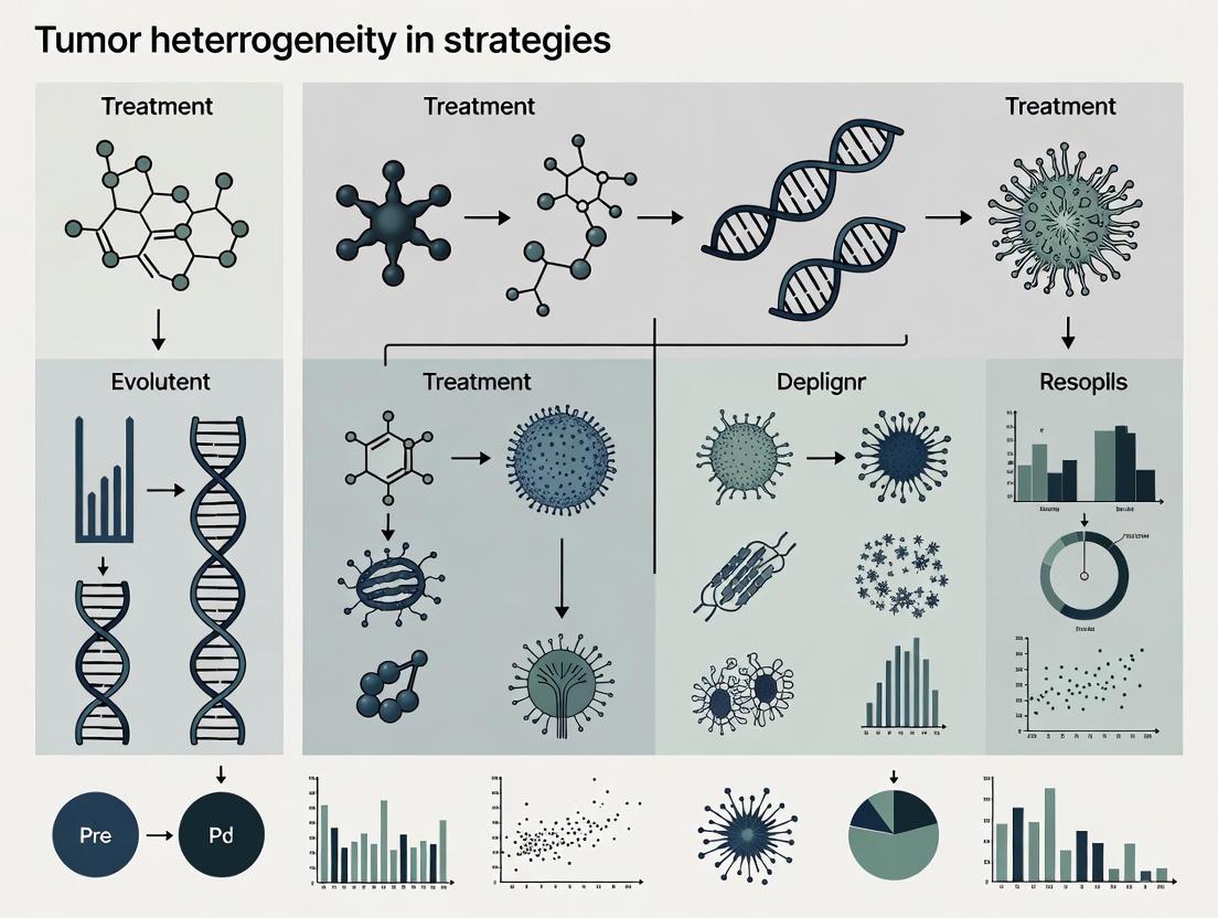
Conquering Cancer Complexity: Advanced Strategies to Overcome Tumor Heterogeneity in Therapeutic Development
This article provides a comprehensive analysis for researchers and drug development professionals on the critical challenge of tumor heterogeneity in oncology.
Conquering Cancer Complexity: Advanced Strategies to Overcome Tumor Heterogeneity in Therapeutic Development
Abstract
This article provides a comprehensive analysis for researchers and drug development professionals on the critical challenge of tumor heterogeneity in oncology. It explores the fundamental biological mechanisms driving intra- and inter-tumoral diversity, examines cutting-edge methodological approaches for characterization and targeting, addresses key hurdles in treatment resistance and biomarker development, and evaluates validation frameworks for novel strategies. By synthesizing foundational concepts with emerging clinical applications, this review aims to bridge the gap between mechanistic understanding and therapeutic innovation, offering a roadmap for developing more effective, heterogeneity-informed cancer treatments.
Decoding the Complex Landscape: Understanding the Biological Basis of Tumor Heterogeneity
Defining Spatial and Temporal Heterogeneity in Solid Tumors
Tumor heterogeneity, the presence of distinct cell subpopulations with different genetic, phenotypic, and behavioral characteristics within a single tumor or between tumors, represents a fundamental challenge in oncology research and therapeutic development [1] [2]. This variability exists across two critical dimensions: spatial heterogeneity (differences across different geographical regions of a single tumor or between primary and metastatic sites) and temporal heterogeneity (changes that occur over time through tumor evolution and in response to therapies) [1] [3]. For researchers and drug development professionals, understanding and accounting for this heterogeneity is crucial for designing effective treatment strategies and avoiding therapeutic resistance.
Spatial heterogeneity manifests as an uneven distribution of tumor cell subpopulations with different molecular characteristics between and within disease sites [1] [3]. Temporal heterogeneity refers to the dynamic changes in cancer cell molecular composition that occur over time, either through natural evolution or in response to selective pressures like drug treatment [1] [3]. These two dimensions of heterogeneity create complex, evolving ecosystems that can confound traditional single-biopsy diagnostic approaches and lead to treatment failure through the selection of resistant subclones.
FAQs: Core Concepts for Researchers
Q1: What are the fundamental mechanisms driving spatial and temporal heterogeneity in solid tumors?
Several interconnected biological mechanisms drive heterogeneity in solid tumors:
- Genomic Instability: Cancer cells exhibit higher mutation rates than normal cells due to defects in DNA repair, telomere maintenance, DNA replication, and chromosome segregation. This creates extensive genetic diversity that serves as the substrate for heterogeneity [1] [4]. The mutation rate per trillion bases across 12 major cancer types ranges from 0.28 to 8.15 [1].
- Clonal Evolution: This Darwinian model proposes that genetically unstable cells accumulate alterations over time, and selective pressures favor the growth and survival of variant subpopulations with a fitness advantage [5] [2]. This can follow linear patterns (successive acquisition of mutations) or, more commonly in solid tumors, branching evolution where multiple genetically distinct populations form from a common ancestor [4].
- Epigenetic Modifications: Changes in DNA methylation, histone modifications, and chromatin remodeling can create stable, heritable phenotypic diversity without altering the DNA sequence itself. Cancer stem cells (CSCs) may generate cellular heterogeneity through epigenetic mechanisms, establishing a differentiation hierarchy within tumors [1] [6].
- Microenvironmental Influences: The tumor microenvironment (TME), including gradients of oxygen, nutrients, and stromal cell interactions (e.g., fibroblasts, immune cells), exerts selective pressures that shape heterogeneity. Variations in blood supply can create distinct niches that favor different subclones [1] [7].
Q2: How does tumor heterogeneity confound biomarker discovery and validation?
Heterogeneity introduces significant challenges in biomarker development:
- Sampling Bias: A single core biopsy or fine needle aspirate may not capture the full spectrum of molecular alterations present in different tumor regions or metastatic sites [5]. For example, in renal cell carcinoma, only about 34% of mutations were consistent across all samples from the same primary tumor and its metastases [1]. This can lead to false-negative results for important biomarkers.
- Temporal Dynamics: A biopsy represents a single moment in a tumor's evolution. The genomic landscape can change substantially over time, particularly under therapeutic selective pressure, meaning diagnostic results can quickly become outdated [1] [5]. For instance, in NSCLC patients treated with EGFR-TKIs, the T790M resistance mutation positivity rate in plasma increases with longer treatment duration [1].
- Incomplete Target Representation: Targeted therapies selected based on a single biopsy may only be effective against a subpopulation of tumor cells, leaving resistant clones to eventually cause disease progression [2].
Q3: What experimental strategies can accurately capture spatial heterogeneity?
To overcome spatial sampling limitations, researchers are employing several advanced strategies:
- Multi-Region Sequencing: Sampling multiple geographically distinct regions from a single tumor during surgical resection provides a more comprehensive genetic profile. For clear cell renal carcinoma, some researchers recommend sampling at least three different regions to ensure accuracy of key mutation tests [1].
- Single-Cell Sequencing: This technology enables the characterization of individual cells within a diverse population, defining complex clonal relationships and revealing rare subpopulations that bulk sequencing would miss [4].
- Radiogenomics and Habitat Imaging: Advanced imaging techniques (MRI, CT, PET/CT) can non-invasively map phenotypic heterogeneity across entire tumors. Quantitative imaging features (radiomics) can be correlated with genomic data to identify region-specific biological characteristics [8].
- Computer Vision and Digital Pathology: Machine learning applied to digitized histology slides can automatically identify and map various cell types (tumor, immune, stromal) across tissue sections, providing quantitative spatial context for cellular interactions within the TME [7].
Q4: How can we effectively monitor temporal heterogeneity throughout disease progression and treatment?
Monitoring temporal heterogeneity requires longitudinal assessment strategies:
- Liquid Biopsies and Circulating Tumor DNA (ctDNA): Serial analysis of ctDNA from blood samples allows for non-invasive, repeated monitoring of clonal dynamics and the emergence of resistance mutations during therapy [9]. This provides a composite snapshot of heterogeneity from multiple tumor sites.
- Serial Biopsies: When feasible and ethically justified, obtaining tumor tissue at key time points (e.g., at progression) can directly reveal evolutionary changes. However, this is invasive and not always possible [5] [2].
- Patient-Derived Model Systems: Establishing patient-derived xenografts (PDXs) or organoids from different time points can preserve and allow functional study of evolving subclones [2].
Troubleshooting Guides: Addressing Common Experimental Challenges
Challenge 1: Inconsistent Results from Different Tumor Regions
Problem: Molecular profiling results (e.g., mutation status, gene expression) vary dramatically between samples taken from different regions of the same tumor, leading to conflicting data.
| Potential Cause | Solution | Key Considerations |
|---|---|---|
| Inadequate sampling | Implement systematic multi-region sampling protocol. For research on surgical specimens, sample from central, peripheral, and intermediate zones, noting spatial coordinates. | Logistically challenging for advanced cancers; sample number must be balanced against tumor size [1]. |
| True extensive spatial heterogeneity | Use imaging-guided biopsy to target regions with distinct radiological features (e.g., hypoxic vs. well-perfused areas). | Requires coordination with radiology department; specialized equipment needed. |
| Analysis of bulk tissue | Employ single-cell sequencing technologies to deconvolute cellular mixtures and identify minority subclones. | Higher cost and computational burden for data analysis [4]. |
Experimental Workflow for Multi-Region Analysis:
- Sample Collection: For resectable tumors, immediately following resection, photograph the specimen and dissect multiple (e.g., 3-5) regions representing different macroscopic appearances (e.g., necrotic core, invasive front, well-defined region).
- Spatial Annotation: Record the precise location of each sample within the tumor. Snap-freeze a portion of each sample in liquid nitrogen and preserve the remainder in formalin for parallel histology.
- Pathological Validation: Perform H&E staining on adjacent sections to confirm tumor content and assess necrosis, immune infiltration, and other histological features for each region.
- DNA/RNA Co-Isolation: Extract nucleic acids from the same tissue piece to enable direct correlation of genomic and transcriptomic data from the same cellular context.
- Parallel Sequencing: Conduct whole-exome or targeted sequencing, and RNA sequencing on all regional samples simultaneously using the same sequencing platform and batch to minimize technical variation.
- Bioinformatic Integration: Use phylogenetic tree analysis to reconstruct evolutionary relationships between regional samples and spatial mapping software to visualize the distribution of clones.
Spatial Heterogeneity Analysis Workflow
Challenge 2: Emergence of Treatment Resistance After Initial Response
Problem: Targeted therapies often produce dramatic initial responses, followed by relapse due to outgrowth of pre-existing or newly acquired resistant subclones.
| Potential Cause | Solution | Key Considerations |
|---|---|---|
| Pre-existing resistant minor subclone | Use highly sensitive NGS assays (e.g., with error correction) on pre-treatment samples to detect low-frequency resistant clones. | Requires deep sequencing coverage; clinical significance of very low-frequency variants may be unclear. |
| Acquired resistance evolution | Implement longitudinal liquid biopsy monitoring (ctDNA) during treatment to track clonal dynamics in real-time. | ctDNA levels can be low in some cancer types; may not capture all resistance mechanisms. |
| Adaptive bypass signaling | Design combination therapies upfront that target primary driver and common resistance pathways simultaneously. | Increased risk of toxicity; requires robust preclinical validation of synergy. |
Protocol for Longitudinal ctDNA Monitoring for Temporal Heterogeneity:
- Baseline Sample Collection: Collect plasma (e.g., 2x10mL Streck tubes) and matched germline DNA (saliva or blood) prior to initiation of therapy.
- Plasma Processing: Process within 6 hours of collection. Centrifuge to isolate plasma, then a second high-speed centrifugation to remove residual cells.
- ctDNA Extraction: Use commercially available circulating nucleic acid kits for extraction.
- Library Preparation and Sequencing: Use NGS panels designed for your cancer type, covering primary driver mutations and known resistance mechanisms. Unique molecular identifiers (UMIs) are critical for error correction and accurate variant calling.
- Schedule for Serial Monitoring: Collect additional plasma samples at defined intervals (e.g., every 4-8 weeks during treatment, and at time of radiographic progression).
- Variant Calling and Clonal Tracking: Bioinformatically identify somatic variants and track their variant allele frequencies (VAFs) over time. Rising VAFs of a specific mutation suggest selective outgrowth of a resistant subclone.
Temporal Heterogeneity Monitoring Approach
Challenge 3: Integrating Complex Heterogeneity Data into Actionable Insights
Problem: Multi-region and single-cell sequencing generate vast, complex datasets that are difficult to interpret and translate into therapeutic strategies.
Solutions and Considerations:
- Computational Clonal Deconvolution: Use bioinformatic tools (e.g., PyClone, SciClone) to estimate the number and prevalence of distinct subclones and their mutational composition from bulk sequencing data of multiple samples [2].
- Phylogenetic Tree Reconstruction: Apply algorithms used in evolutionary biology to infer the ancestral relationships between different tumor subclones, distinguishing early "truncal" events (present in all subclones) from later "branch" events (private to specific subclones) [2].
- Functional Validation of Targets: Prioritize therapeutic targeting of "truncal" mutations present in all subclones. For branch-specific resistance mutations, use in vitro models (e.g., CRISPR-engineered isogenic cell lines) to confirm functional impact and drug sensitivity.
The Scientist's Toolkit: Research Reagent Solutions
The following table details essential reagents and technologies for studying tumor heterogeneity.
| Research Tool | Primary Function | Key Application in Heterogeneity Research |
|---|---|---|
| Next-Generation Sequencing (NGS) [1] [5] | High-throughput DNA/RNA sequencing. | Comprehensive profiling of genetic alterations across multiple tumor regions or time points. |
| Single-Cell RNA Sequencing (scRNA-seq) [4] | Transcriptome profiling of individual cells. | Deconvoluting cellular composition, identifying rare cell states, and reconstructing trajectories of cellular differentiation and plasticity within tumors. |
| Liquid Biopsy Kits (ctDNA extraction) | Isolation of cell-free DNA from blood plasma. | Non-invasive longitudinal monitoring of clonal dynamics and emergence of resistance mutations during therapy [9]. |
| Multiplex Immunofluorescence (mIF) | Simultaneous detection of multiple protein markers on a single tissue section. | Spatial profiling of the tumor immune microenvironment, revealing interactions between specific tumor subclones and immune cell populations [7]. |
| Patient-Derived Organoids (PDOs) | 3D ex vivo cultures derived from patient tumor tissue. | Functional testing of drug sensitivity on a patient-specific basis, potentially capturing some of the original tumor's heterogeneity [2]. |
| Unique Molecular Identifiers (UMIs) | Short random nucleotide sequences added to each DNA fragment during library prep. | Error correction in NGS data, enabling accurate detection of low-frequency variants critical for identifying minor subclones. |
| Digital Pathology Software [7] | Machine learning-based image analysis of whole slide images. | Quantitative analysis of spatial relationships between different cell types, and identification of histologically distinct regions for targeted sampling. |
The table below consolidates quantitative findings from studies on tumor heterogeneity, providing reference points for researchers designing and interpreting experiments.
| Metric | Value / Range | Context / Implication | Reference |
|---|---|---|---|
| Spatial Heterogeneity (Mutation Concordance) | ~34% | Proportion of mutations found consistently across all regions of a primary renal tumor and its metastases. Highlights extensive spatial divergence. | [1] |
| Driver Mutation Heterogeneity in NSCLC | >75% | Proportion of tumor driver mutations that were heterogeneous (not present in all regions) in early-stage NSCLC. | [1] |
| Range of Mutation Rates | 0.28 - 8.15 per megabase | The variation in mutation rates found across 12 major categories of cancer, underlying the variable substrate for heterogeneity. | [1] |
| Oncogenic Driver Detection Rate | 64% | Proportion of 733 lung cancer patients in the LCMC study whose tumors had a detectable oncogenic driver. | [5] |
| Average Genomic Alterations in NSCLC | 10.8 per sample | The average number of genomic alterations found per sample in an NGS study of 364 NSCLC patients, indicating inherent complexity. | [5] |
Addressing spatial and temporal heterogeneity is not merely a technical challenge but a paradigm shift in cancer research. Moving forward, successful therapeutic strategies will need to be inherently dynamic and multi-faceted. This includes the development of rational combination therapies that target both truncal drivers and common resistance pathways, the integration of liquid biopsies into clinical trial designs for real-time adaptive therapy, and a greater focus on targeting the tumor ecosystem itself—including the immune compartment and stromal elements—to reduce the adaptive capacity of heterogeneous tumors. By adopting the sophisticated sampling, analytical, and monitoring tools outlined in this guide, researchers can deconstruct heterogeneity from an obstacle into a roadmap for designing more durable and effective cancer treatments.
Foundational Concepts & Frequently Asked Questions
Q1: How do the Clonal Evolution and Cancer Stem Cell (CSC) models explain tumor heterogeneity, and are they mutually exclusive?
A: The Clonal Evolution model posits that tumors are a mosaic of subpopulations of cells that have accumulated diverse mutations over time. Darwinian selection acts on this genetic diversity, favoring the expansion of clones with a fitness advantage (e.g., faster proliferation or resistance to therapy) within a given microenvironment [10]. In contrast, the CSC model proposes a hierarchical organization where only a small subset of cells, the CSCs, possess the ability to self-renew and differentiate into the heterogeneous lineages of cancer cells that constitute the tumor [10].
These models are not mutually exclusive. Evidence suggests that CSCs themselves can be a product of clonal evolution. Somatic evolution can select for cancer cells that acquire "stemness" traits, such as upregulation of drug-efflux proteins and pro-survival signaling pathways, which impart a significant fitness advantage. Therefore, clonal selection for stem cell characteristics may result in the emergence of CSCs within a tumor [10].
Q2: What are the key practical implications of these models for therapy and drug resistance?
A: The two models have distinct but overlapping implications for treatment failure:
- Clonal Evolution: Drug resistance arises from the pre-existence or spontaneous development of genetically resistant subclones. Treatment acts as a selective pressure, eliminating sensitive cells and allowing resistant clones to expand. This resistance is typically irreversible as it is genetically encoded [11].
- Cancer Stem Cell: CSCs are often inherently resistant to conventional therapies due to properties like quiescence, enhanced DNA repair, and expression of drug-efflux pumps (e.g., ABC transporters). Eradicating the CSC population is considered crucial for achieving long-term remission, as they can regenerate the tumor. Resistance can also involve reversible, non-genetic plasticity, where cells change their functional state to adapt to therapeutic pressure [10] [11].
Modern treatment strategies must account for both irreversible genetic resistance and reversible cellular plasticity [11].
Q3: How is intratumoral heterogeneity investigated experimentally?
A: Key methodologies include:
- Single-Cell RNA Sequencing (scRNA-seq): This powerful technique allows researchers to profile the transcriptomes of individual cells within a tumor, revealing distinct cell subtypes, states, and lineage relationships. It is instrumental in classifying molecular subtypes and understanding cellular plasticity [12] [13].
- Patient-Derived Xenografts (PDXs): Transplanting patient tumor tissue into immunodeficient mice preserves the original tumor's heterogeneity and architecture. PDX models are used to study tumor growth, metastasis, and therapy response in a context that closely mimics the patient's disease [12].
- Mathematical Modeling: Computational frameworks simulate the population dynamics of tumor subclones and their response to treatments. These models can incorporate both genetic evolutionary dynamics and non-genetic plasticity to predict optimal therapeutic sequences and combat resistance [11].
Key Quantitative Data
Table 1: Frequently Mutated Cancer Gene Categories Across Human Cancers (Analysis of 20,331 tumors, 41 cancer types) [14]
| Gene Category | Example Genes | Percentage of Tumors with Mutations in Category |
|---|---|---|
| Tumor Suppressor Genes | TP53, PTEN, CSMD3 | 94% |
| Oncogenes | KRAS, PIK3CA, MUC16 | 93% |
| Transcription Factors | TP53, KMT2C | 72% |
| Kinases | PIK3CA, BRAF, ATM | 64% |
| Cell Surface Receptors | MUC16, LRP1B | 63% |
| Phosphatases | PTPRT, PTEN | 22% |
Table 2: Molecular Subtypes of Small Cell Lung Cancer (SCLC) and Their Characteristics [12]
| Subtype | Defining Transcription Factor | Key Characteristics | Therapeutic Implications |
|---|---|---|---|
| SCLC-A | ASCL1 | High neuroendocrine (NE) differentiation; classic floating aggregates. | More susceptible to first-line chemotherapy (cisplatin). |
| SCLC-N | NEUROD1 | High neuroendocrine differentiation; more prevalent in lymph node/distant metastases. | More susceptible to first-line chemotherapy (cisplatin). |
| SCLC-P | POU2F3 | Non-neuroendocrine; adherent cell morphology; may undergo EMT. | Potential target for novel therapies. |
| SCLC-I | (Inflammatory) | Low ASCL1/NEUROD1/POU2F3; high inflammatory/immune markers. | More responsive to immunotherapy (PD-1/PD-L1 inhibitors). |
Experimental Protocols
Protocol 1: Investigating Tumor Heterogeneity and Subtype Plasticity Using scRNA-seq
Application: Classifying molecular subtypes of a tumor (e.g., SCLC) and tracking subtype shifts in response to therapy [12] [13].
- Sample Preparation: Obtain fresh tumor tissue from a primary or metastatic site. For therapy response studies, collect paired samples (pre- and post-treatment).
- Single-Cell Suspension: Dissociate the tissue into a single-cell suspension using mechanical and enzymatic (e.g., collagenase) digestion. Filter through a cell strainer to remove clumps.
- scRNA-seq Library Preparation: Use a platform like the 10x Genomics Chromium to capture individual cells, barcode their RNA, and prepare sequencing libraries.
- Sequencing & Data Processing: Perform high-throughput sequencing on an Illumina platform. Align sequences to a reference genome and generate a gene expression matrix (cells x genes).
- Bioinformatic Analysis:
- Quality Control: Filter out low-quality cells (high mitochondrial gene percentage, low unique gene counts).
- Clustering & Visualization: Use dimensionality reduction techniques (PCA, UMAP) and graph-based clustering (e.g., Seurat, Scanpy) to identify distinct cell populations.
- Subtype Annotation: Identify clusters based on the expression of known marker genes (e.g., ASCL1 for SCLC-A, POU2F3 for SCLC-P, CD3D for T-cells).
- Trajectory Inference: Apply algorithms (e.g., Monocle, PAGA) to infer potential lineage relationships and plasticity between subtypes.
Protocol 2: Evaluating Treatment Efficacy and Resistance In Vivo Using PDX Models
Application: Testing personalized treatment sequences and monitoring the emergence of resistant subclones [12] [11].
- Model Generation: Implant patient-derived tumor fragments or cells subcutaneously or orthotopically into immunodeficient mice (e.g., NSG mice).
- Treatment Cohorts: Once tumors are established (e.g., ~100-150 mm³), randomize mice into different treatment arms (e.g., Drug A, Drug B, combination, sequential therapy, or vehicle control).
- Treatment and Monitoring: Administer therapies according to the designated schedule. Measure tumor volumes and mouse weights 2-3 times per week.
- Endpoint Analysis:
- Harvest Tumors: At the end of the study, harvest tumors from all cohorts.
- Downstream Applications: Analyze tumors via:
- Genomic DNA sequencing to track the evolution of specific genetic subclones.
- scRNA-seq (as in Protocol 1) to profile cellular heterogeneity and identify shifts in subtype composition post-treatment.
- IHC/Flow Cytometry to validate protein-level markers of resistance or subtype identity.
The Scientist's Toolkit: Essential Research Reagents & Materials
Table 3: Key Reagents for Investigating Genetic Drivers and Heterogeneity
| Item | Function/Application |
|---|---|
| Collagenase/Hyaluronidase | Enzymatic digestion of solid tumor tissue to create single-cell suspensions for scRNA-seq or flow cytometry [13]. |
| Fetal Bovine Serum (FBS) | Essential component of cell culture media for growing and maintaining patient-derived cells or established cancer cell lines. |
| Matrigel | Basement membrane extract used for 3D cell culture (organoids) and to support the engraftment and growth of PDX models. |
| DMSO (Cryopreservation Medium) | Used for the cryopreservation of viable tumor cells, organoids, and tumor fragments for long-term storage and biobanking. |
| Antibodies for Flow Cytometry (e.g., anti-CD44, anti-CD133) | Used to identify and isolate potential Cancer Stem Cell populations via Fluorescence-Activated Cell Sorting (FACS). |
| CellTiter-Glo Luminescent Assay | A homogeneous method used to determine the number of viable cells in culture based on quantitation of ATP, useful for drug screening. |
| TRIzol Reagent | A monophasic solution of phenol and guanidine isothiocyanate for the isolation of high-quality total RNA from cells and tissues for sequencing. |
Signaling Pathways & Experimental Workflows
Treatment Resistance Logic
SCLC Analysis Workflow
Troubleshooting Guides
Guide 1: Investigating Epigenetic Drug Tolerance in Cell Models
Problem: A subset of cancer cells survives initial drug treatment, showing no genetic mutations, suggesting a non-genetic, reversible resistance.
Investigation Framework:
- Confirm Non-Genetic Basis: Perform whole-exome sequencing on parental and drug-tolerant persister (DTP) cells to rule out acquired genetic mutations [15].
- Profile Epigenetic State: Use chromatin immunoprecipitation sequencing (ChIP-seq) for histone marks (e.g., H3K4me3, H3K27me3) and whole-genome bisulfite sequencing (WGBS) for DNA methylation in both cell populations [16] [17].
- Test for Phenotypic Plasticity:
- Conduct a drug withdrawal assay; non-genetic resistance often leads to re-sensitization after several cell divisions in a drug-free medium [15].
- Use single-cell RNA sequencing (scRNA-seq) to identify distinct cellular states (e.g., stem-like, mesenchymal) and their transitions upon drug pressure [18].
- Identify Key Epigenetic Regulators: Perform a functional CRISPR screen targeting epigenetic "writers," "readers," and "erasers" in DTP cells to identify enzymes essential for survival [16] [17].
Solution: The acquired resistance is likely stable non-genetic resistance mediated by heritable epigenetic reprogramming. Combination therapy with an epigenetic drug (e.g., DNMT or EZH2 inhibitor) and the original anticancer agent may prevent or reverse this resistance [16] [15].
Guide 2: Overcoming Resistance to KRAS G12C Inhibitors
Problem: Non-small cell lung cancer (NSCLC) patients develop resistance to KRAS G12C inhibitors (e.g., sotorasib, adagrasib) without secondary genetic mutations in ~50% of cases [19].
Investigation Framework:
- Analyse Protein Interaction Networks: Use co-immunoprecipitation followed by mass spectrometry to investigate if drug binding alters KRAS conformational dynamics and rewires its interactions with partner proteins [19].
- Assess Transcriptional Reprogramming: Perform RNA-seq on resistant cells to identify upregulated bypass signaling pathways (e.g., RTK, MAPK) [19].
- Evaluate Phenotypic Plasticity: Use flow cytometry to track markers of cellular differentiation states; resistance is frequently associated with a shift towards a stem-like or de-differentiated phenotype [15].
Solution: Resistance emerges from a nexus of non-genetic and genetic mechanisms. A combination of KRAS G12C inhibitors with other agents is a primary strategy. Preclinical data suggests that combining sotorasib with the proteasome inhibitor carfilzomib can alleviate this resistance [19].
Frequently Asked Questions (FAQs)
FAQ 1: What is the difference between genetic and non-genetic drug resistance in cancer?
Answer: Genetic resistance is caused by permanent mutations in the DNA sequence that are selectively amplified under treatment pressure. In contrast, non-genetic resistance involves reversible changes in gene expression that do not alter the underlying DNA sequence. This is often driven by epigenetic modifications (e.g., DNA methylation, histone modifications) and phenotypic plasticity, allowing cancer cells to dynamically switch between drug-sensitive and drug-tolerant states [15].
FAQ 2: How does phenotypic plasticity contribute to therapy failure?
Answer: Phenotypic plasticity is the ability of a cancer cell to change its identity and functional state in response to environmental cues, such as drug treatment. For example, in Glioblastoma (GBM), standard chemo-radiation therapy can reprogram non-stem tumor cells to acquire stem-like characteristics (de-differentiation) or transdifferentiate into vascular-like cells. This plasticity generates cellular heterogeneity and fosters the outgrowth of therapy-resistant cell populations that drive tumor recurrence [18].
FAQ 3: What are the main epigenetic mechanisms driving this plasticity and resistance?
Answer: The core mechanisms, which are frequently dysregulated in cancer, are summarized in the table below.
Table 1: Key Epigenetic Mechanisms in Cancer Therapy Resistance
| Mechanism | Description | Role in Resistance |
|---|---|---|
| DNA Methylation | Addition of methyl groups to cytosine bases in DNA, typically leading to gene silencing. | Hypermethylation of tumor suppressor gene promoters (e.g., P16, RASSF1A) silences them, aiding cell survival. Global hypomethylation can cause genomic instability and oncogene activation [16] [20] [21]. |
| Histone Modifications | Post-translational changes (e.g., acetylation, methylation) to histone proteins that alter chromatin structure. | Alterations in marks like H3K27ac (activation) and H3K27me3 (repression) reprogram the transcriptome, promoting survival and stemness. For instance, radiation can induce histone modifications that drive a proneural-to-mesenchymal transition in GBM, increasing invasiveness and resistance [16] [18]. |
| RNA Modifications (Epitranscriptomics) | Chemical modifications to RNA molecules, such as N6-methyladenosine (m6A), that regulate their fate. | m6A modifications impact RNA stability and translation of key transcripts involved in drug metabolism, DNA repair, and cellular survival pathways [16] [20]. |
| Non-coding RNAs (ncRNAs) | RNA molecules that do not code for proteins but regulate gene expression (e.g., miRNAs, lncRNAs). | ncRNAs can function as master regulators, fine-tuning the expression of entire networks of genes involved in cell death, proliferation, and stemness, thereby modulating the tumor's response to therapy [16] [21]. |
FAQ 4: Can non-genetic resistance become stable and heritable?
Answer: Yes. While some forms like drug-tolerant persisters (DTPs) are transient, non-genetic changes can lead to stable, mitotically active resistance. This occurs through epigenetic heterogeneity and selection, where pre-existing or induced cell subpopulations with stable, heritable epigenetic states that confer resistance are expanded under therapeutic pressure [15].
Experimental Protocols & Data
Protocol 1: Generating and Characterizing Drug-Tolerant Persister (DTP) Cells
Purpose: To establish a model of reversible, non-genetic drug resistance in vitro [15].
Materials:
- Cancer cell line of interest
- Cytotoxic or targeted anticancer drug
- Cell culture reagents and equipment
Method:
- DTP Induction: Treat a confluent monolayer of cancer cells with a high concentration of the drug (e.g., 10x IC50) for an extended period (e.g., 5-9 days). Include a DMSO vehicle control.
- DTP Isolation: After treatment, a small fraction of surviving, non-proliferating cells will remain adherent. Wash and maintain these cells in fresh drug-containing media; these are the DTPs.
- Characterization:
- Reversibility Assay: Wash DTPs and culture them in drug-free media. Monitor for regrowth and re-test drug sensitivity after 2-3 weeks to confirm re-sensitization.
- Molecular Profiling: Extract RNA and protein from DTPs and parental cells for transcriptomic (RNA-seq) and proteomic analysis to identify upregulated resistance pathways.
Protocol 2: Assessing DNA Methylation Status via Bisulfite Sequencing
Purpose: To map genome-wide DNA methylation patterns and identify hyper/hypomethylated regions associated with resistance [20] [17].
Materials:
- Genomic DNA from sensitive and resistant cells
- Bisulfite conversion kit (e.g., EZ DNA Methylation Kit)
- Next-generation sequencing platform and bioinformatics tools
Method:
- Bisulfite Conversion: Treat 500 ng - 1 µg of genomic DNA with sodium bisulfite. This converts unmethylated cytosines to uracils (which are read as thymines in sequencing), while methylated cytosines remain unchanged.
- Library Prep & Sequencing: Prepare a sequencing library from the converted DNA and run on an NGS platform.
- Bioinformatic Analysis:
- Align sequences to a bisulfite-converted reference genome.
- Calculate methylation percentage per cytosine as
# reads with 'C' / (# reads with 'C' + # reads with 'T'). - Identify Differentially Methylated Regions (DMRs) between sensitive and resistant cells, focusing on promoter CpG islands.
Table 2: Quantitative Data on KRAS G12C Inhibitor Combination Trials
| Combination Therapy | Clinical Trial | Response Rate | Key Finding |
|---|---|---|---|
| Adagrasib + Pembrolizumab (anti-PD1) | KRYSTAL-1 / KRYSTAL-7 | 49% - 57% | Combination was well-tolerated, but response rates were not significantly improved over monotherapy in some contexts [19]. |
| Sotorasib + Trametinib (MEK inhibitor) | CodeBreak 101 | 20% (sotorasib-naïve); 0% (sotorasib-resistant) | The combination showed limited efficacy, particularly in patients with prior resistance to KRAS inhibition [19]. |
Signaling Pathways and Workflows
Therapy-Induced Plasticity
DTP Investigation Workflow
The Scientist's Toolkit
Table 3: Research Reagent Solutions for Epigenetic Plasticity Studies
| Item | Function/Brief Explanation | Example Application |
|---|---|---|
| DNMT Inhibitors (e.g., 5-Azacytidine, Decitabine) | Inhibit DNA methyltransferases (DNMTs), causing passive DNA demethylation and reactivation of silenced genes. | Test if reversing promoter hypermethylation re-sensitizes resistant cells to therapy [16] [21]. |
| HDAC Inhibitors (e.g., Vorinostat, Panobinostat) | Inhibit histone deacetylases (HDACs), leading to increased histone acetylation and a more open, transcriptionally permissive chromatin state. | Use in combination with other agents to disrupt the epigenetic state that maintains resistance [16]. |
| EZH2 Inhibitors (e.g., Tazemetostat) | Inhibit EZH2, the catalytic subunit of PRC2, which is responsible for depositing the repressive H3K27me3 mark. | Target the epigenetic maintenance of a stem-like or de-differentiated state in resistant cells [16] [18]. |
| Bisulfite Conversion Kits | Chemically modify DNA for downstream analysis, distinguishing methylated from unmethylated cytosines. | Prepare samples for whole-genome bisulfite sequencing to map DNA methylation patterns [20] [17]. |
| ChIP-Grade Antibodies | Highly specific antibodies for immunoprecipitating DNA-protein complexes. Essential for ChIP-seq. | Perform ChIP-seq for histone marks (e.g., H3K4me3, H3K27ac, H3K27me3) to map the chromatin landscape [16] [17]. |
| Single-Cell RNA-Seq Kits | Enable transcriptome profiling at the single-cell level to resolve cellular heterogeneity and state transitions. | Identify rare subpopulations (e.g., DTPs) and trace lineage trajectories during acquired resistance [18]. |
The Tumor Microenvironment's Role in Shaping Heterogeneity
Frequently Asked Questions & Troubleshooting Guides
Q1: Why does my preclinical drug candidate show efficacy in vitro but fail in animal models, and how can TME heterogeneity explain this?
A: This common failure often stems from the inability of simple in vitro models to capture the complex cellular interactions and physical barriers present in actual tumor microenvironments. 2D cell lines lack the three-dimensional architecture and cellular diversity of real tumors [22].
Troubleshooting Steps:
- Implement advanced models: Transition to more physiologically relevant models such as Patient-Derived Organoids and Patient-Derived Xenografts that better preserve original tumor characteristics and some TME components [22].
- Analyze spatial relationships: Use multiplex immunohistochemistry to determine if your drug target is located in inaccessible tumor regions (e.g., surrounded by dense fibrosis) [23].
- Profile TME composition: Characterize the model's CAF subpopulations, immune cell infiltration, and extracellular matrix composition using single-cell RNA sequencing to identify potential resistance mechanisms [24] [25].
Q2: How can I determine if observed drug resistance is due to pre-existing tumor cell heterogeneity or TME-mediated adaptation?
A: Distinguishing between these resistance mechanisms requires integrated analysis of both cancer cell-intrinsic factors and microenvironmental influences over time.
Experimental Approach:
- Establish baseline heterogeneity: Perform single-cell RNA sequencing on untreated control samples to identify pre-existing subpopulations with different transcriptional profiles (e.g., mesenchymal-like, luminal-like, basal-like cells) [26].
- Track clonal dynamics: Use barcoding technologies or CNV analysis to monitor how different subclones expand or contract during treatment [26] [27].
- Correlate with TME changes: Analyze parallel changes in stromal and immune cell composition using the same single-cell data to identify TME factors associated with resistant subclones [26] [25].
Table 1: Key Analytical Methods for Investigating Resistance Mechanisms
| Method | Application | Technical Considerations |
|---|---|---|
| Single-cell RNA sequencing | Simultaneous profiling of malignant and stromal cell populations; identification of pre-existing and emergent subpopulations | Requires fresh or properly preserved tissue; computational expertise needed for data analysis [26] [25] |
| Multiplex immunohistochemistry (IHC) | Spatial analysis of protein expression in intact tissue architecture; cell-cell interaction studies | Panel design crucial; antibody validation required; tissue morphology preservation [23] [27] |
| Spatial transcriptomics | Mapping gene expression to tissue locations; correlation of heterogeneity with histological features | Lower resolution than single-cell; integration with H&E staining recommended [25] |
| Patient-Derived Xenografts (PDX) | Study of human tumors in in vivo context while preserving some TME components; drug response studies | Immune-deficient hosts limit immune interactions; stromal cells eventually replaced by mouse cells [22] |
Q3: What biomarkers can I use to enrich patient populations for early-phase immunotherapy trials to avoid false negative results?
A: The Society for Immunotherapy of Cancer recommends biomarker-based enrichment strategies to increase the likelihood of detecting clinical signals in early-phase trials [28].
Enrichment Framework:
- For T-cell-targeting agents: Start with CD8+ IHC to identify tumors with T-cell infiltration, then retrospectively develop more precise biomarkers using multiomics [28].
- For non-T-cell targeting agents: Select enrichment biomarkers based on preclinical data showing pathway modulation, such as:
- Tertiary lymphoid structures (CD20+ B cells)
- Myeloid cells (CD68+, CD163+)
- Fibroblast subsets
- Neutrophil-to-lymphocyte ratio [28]
Table 2: TME-Based Biomarkers for Patient Enrichment in Clinical Trials
| Biomarker Category | Specific Markers | Detection Method | Enrichment Context |
|---|---|---|---|
| T-cell Inflammation | CD8+, CD3+, PD-L1 | IHC, multiplex IHC | ICIs, T-cell engagers [28] [27] |
| Myeloid Cells | CD68 (macrophages), CD163 (M2-like TAMs) | IHC, flow cytometry | Myeloid-targeting agents [28] |
| Tertiary Lymphoid Structures | CD20+ B cells, DC-LAMP+ dendritic cells | Multiplex IHC, H&E | Prognostic assessment, response prediction [28] |
| Cancer-Associated Fibroblasts | α-SMA, FAP, PDGFRβ | IHC, single-cell RNA-seq | Stroma-modifying therapies [24] [25] |
| Tumor Mutational Burden | Whole exome sequencing | NGS | ICIs in certain cancer types [28] |
Q4: How can I account for spatial heterogeneity when analyzing biopsy samples for clinical trial stratification?
A: Spatial heterogeneity presents significant challenges for accurate biomarker assessment, as single biopsies may not represent the entire tumor's biology [27].
Best Practices:
- Multi-region sampling: Obtain 3-5 core biopsies from different tumor regions when possible, avoiding fine needle aspirations which disrupt architecture [28].
- Prioritize recent metastases: When studying advanced disease, sample metastases rather than primary tumors when feasible, as TME composition differs significantly [27].
- Implement digital pathology: Use automated analysis to quantify cell densities and spatial relationships (e.g., immune cell proximity to cancer cells) across entire tissue sections [23] [27].
Experimental Protocols
Protocol 1: Comprehensive TME Profiling Using Multiplex Immunohistochemistry
Purpose: Simultaneous characterization of multiple immune and stromal cell populations while preserving spatial information.
Materials:
- Formalin-fixed, paraffin-embedded (FFPE) tissue sections (3-5 μm)
- Validated antibody panel (e.g., 9-17 markers covering T cells, B cells, myeloid cells, checkpoint markers, structural markers)
- Orion platform or comparable multiplex IHC system
- Image analysis software with cellular neighborhood analysis capability [23]
Method:
- Tissue preparation: Cut sections, deparaffinize, and perform antigen retrieval.
- Staining cycles: For each marker, apply primary antibody, secondary detection, fluorescence-conjugated tyramide signal amplification, and antibody stripping.
- Image acquisition: Scan slides using high-resolution fluorescence scanner.
- Image analysis:
- Segment individual cells based on nuclear and membrane markers
- Assign cell phenotypes based on marker combinations
- Perform spatial cellular graph partitioning to identify cellular neighborhoods
- Calculate cell-cell proximity metrics [23]
Troubleshooting:
- High background: Optimize antibody concentrations and stripping conditions
- Signal loss: Validate antibody compatibility with stripping protocol
- Analysis errors: Manually review a subset of cell classifications for accuracy
Protocol 2: Single-Cell RNA Sequencing to Decipher TME Heterogeneity
Purpose: Deconvolute cellular composition of tumors and identify novel cell subpopulations associated with therapy resistance.
Materials:
- Fresh tumor tissue or properly preserved tissue (RNAlater or snap-frozen)
- Single-cell RNA sequencing platform (10X Genomics, Drop-seq, etc.)
- Cell viability >80% recommended
- Bioinformatics pipeline for scRNA-seq analysis [26] [25]
Method:
- Single-cell suspension: Dissociate tissue using gentle enzymatic digestion (collagenase/hyaluronidase) with minimal processing time.
- Cell sorting: Remove dead cells and debris using flow cytometry or microfluidic devices.
- Library preparation: Use chosen platform to barcode individual cells and prepare sequencing libraries.
- Sequencing: Aim for 50,000 reads per cell as a minimum.
- Bioinformatic analysis:
- Quality control (remove cells with high mitochondrial gene percentage)
- Normalization and integration of multiple samples
- Unsupervised clustering and cell type annotation using canonical markers
- Trajectory inference and differential expression analysis
- Cell-cell communication network inference [26] [25]
Troubleshooting:
- Low cell viability: Optimize dissociation protocol; use viability enhancers
- Doublets: Adjust cell concentration loading; use computational doublet detection
- Batch effects: Include sample multiplexing and use integration algorithms
Research Reagent Solutions
Table 3: Essential Research Tools for TME Heterogeneity Studies
| Reagent/Tool Category | Specific Examples | Primary Function | Key Considerations |
|---|---|---|---|
| Multiplex IHC Panels | 17-plex tumor immune landscape assay (CD3, CD8, CD20, CD68, CD163, PD-1, PD-L1, etc.) | Comprehensive spatial profiling of immune and stromal cells | Requires validated antibody compatibility; specialized imaging platforms [23] |
| Single-Cell Analysis Platforms | 10X Genomics, BD Rhapsody | High-throughput single-cell transcriptomic profiling | Cell viability critical; computational expertise required [26] [25] |
| Spatial Transcriptomics | 10X Visium, Nanostring GeoMx | Mapping gene expression to tissue locations | Integration with H&E staining; resolution limitations [25] |
| Preclinical Models | Patient-Derived Organoids, Patient-Derived Xenografts | Drug testing in context preserving some TME features | PDX models lose human stroma over time; organoids lack full TME [22] |
| Computational Tools | TMEtyper, CARD, inferCNV | Deciphering cellular composition from bulk or spatial data | Algorithm selection depends on research question and data type [29] [25] |
Visualizing Key Concepts
Diagram 1: Tumor Microenvironment Heterogeneity and Therapeutic Implications
Diagram 2: Integrated Workflow for TME Heterogeneity Analysis
Small cell lung cancer (SCLC) has undergone a significant paradigm shift, from being considered a single disease entity to a malignancy comprising distinct molecular subtypes with unique therapeutic vulnerabilities. This transformation is largely driven by the discovery of lineage-defining transcription factors that orchestrate different transcriptional programs. The current consensus classification system defines four primary subtypes: SCLC-A (ASCL1-dominant), SCLC-N (NEUROD1-dominant), SCLC-P (POU2F3-dominant), and SCLC-I (inflamed) [30] [12] [31].
This classification system provides a critical framework for addressing the profound tumor heterogeneity that characterizes SCLC and enables the development of precision medicine approaches. Understanding these subtypes, their biological drivers, and their dynamic nature is essential for designing effective therapeutic strategies and overcoming treatment resistance [30] [12].
Molecular Subtypes of SCLC
Subtype Characteristics and Prevalence
SCLC subtypes demonstrate distinct transcriptional profiles, cellular origins, and clinical behaviors. The table below summarizes the key characteristics of each major subtype.
Table 1: Molecular Subtypes of Small Cell Lung Cancer
| Subtype | Defining Transcription Factor | Approximate Prevalence | Key Characteristics | Cell of Origin |
|---|---|---|---|---|
| SCLC-A | ASCL1 | ~70% [30] | Neuroendocrine-high; expresses MYCL, SOX2, DLL3, BCL2 [30] | Pulmonary neuroendocrine cells [32] |
| SCLC-N | NEUROD1 | ~15% [30] | Neuroendocrine-high; associated with MYC expression and aggressive phenotype [30] | Pulmonary neuroendocrine cells [32] |
| SCLC-P | POU2F3 | 7-15% [30] | Non-neuroendocrine; tuft cell lineage; expresses SOX9, ASCL2, IGFR1 [30] | Tuft cells [32] |
| SCLC-I | Low ASCL1/NEUROD1/POU2F3; High inflammatory markers [12] | Not firmly established | Non-neuroendocrine; immune-enriched gene signature [12] | Various, including club and AT2 cells [32] |
Detailed Subtype Profiles and Therapeutic Vulnerabilities
Each SCLC subtype possesses unique molecular dependencies that present opportunities for targeted therapeutic intervention.
Table 2: Subtype-Specific Therapeutic Vulnerabilities and Biomarkers
| Subtype | Key Biomarkers | Therapeutic Vulnerabilities | Response to Therapy |
|---|---|---|---|
| SCLC-A | ASCL1, DLL3, BCL2, INSM1 [30] [12] | DLL3-targeting agents (e.g., Tarlatamab), BCL2 inhibitors [30] | More responsive to cisplatin; susceptible to ASCL1-targeting approaches [30] [12] |
| SCLC-N | NEUROD1, MYC, AURKA/B, OTX2 [30] | Aurora kinase inhibitors, BET inhibitors [30] | Associated with chemotherapy resistance; Aurora kinase inhibition potential [30] |
| SCLC-P | POU2F3, SOX9, ASCL2, IGFR1 [30] | IGF1R inhibitors, PARP inhibitors (due to DNA repair deficiencies) [30] | Susceptible to IGF1R-targeted therapies and DNA-damaging agents [30] |
| SCLC-I | HLA genes, IFNγ-related genes, immune checkpoints [12] [31] | Immune checkpoint inhibitors (e.g., anti-PD-L1) [12] | Better response to immunotherapy; greatest benefit from ICB in NE-SCLC-I subset [12] [31] |
Experimental Workflows for SCLC Subtyping
Molecular Subtyping Workflow
The following diagram illustrates the comprehensive workflow for molecular subtyping of SCLC, integrating multiple omics technologies and analytical approaches.
Diagram 1: Comprehensive SCLC molecular subtyping workflow integrating multi-omics data and functional validation.
Key Methodologies for Subtype Identification
Transcriptomic Profiling: Bulk RNA sequencing remains the foundational method for initial subtype classification based on expression of lineage-defining transcription factors (ASCL1, NEUROD1, POU2F3) and inflammatory markers [30] [31]. For studies requiring single-cell resolution, single-cell RNA sequencing (scRNA-seq) is recommended to assess intratumoral heterogeneity and subtype plasticity [12] [31].
Computational Analysis: Apply non-negative matrix factorization (NMF) to RNA-seq data from patient tumors to identify coherent molecular subtypes. This unsupervised approach has been instrumental in defining the SCLC-I subtype based on inflammatory gene signatures [31]. Validate subtype calls using established transcriptional signatures from reference datasets [30] [31].
Experimental Validation: Utilize patient-derived xenograft (PDX) models, cell-derived xenografts (CDXs), and genetically engineered mouse models (GEMMs) to confirm subtype-specific vulnerabilities and investigate mechanisms of therapy resistance [32] [31]. These models are particularly valuable for studying subtype plasticity and dynamic subtype transitions in response to therapeutic pressure [12] [31].
Research Reagent Solutions
Table 3: Essential Research Reagents for SCLC Subtype Investigation
| Reagent/Category | Specific Examples | Research Application |
|---|---|---|
| Cell Line Models | SCLC-A: H82, H69; SCLC-N: H196, H187; SCLC-P: H2172; SCLC-Y: H1184 [30] [31] | In vitro studies of subtype-specific biology and drug screening |
| Animal Models | Genetically engineered mouse models (GEMMs), Patient-derived xenografts (PDXs) [32] [31] | In vivo validation of subtypes and therapeutic efficacy |
| Antibodies for IHC | Anti-ASCL1, Anti-NEUROD1, Anti-POU2F3, Anti-YAP1, Anti-DLL3 [30] [12] | Subtype identification in tissue sections |
| Targeted Inhibitors | BCL-2 inhibitors (Venetoclax), Aurora kinase inhibitors, PARP inhibitors, IGF1R inhibitors [30] | Functional studies of subtype-specific vulnerabilities |
| qPCR Assays | TaqMan assays for ASCL1, NEUROD1, POU2F3, INSM1, DLL3, AURKA, immune markers [30] [12] | Rapid subtype verification and biomarker quantification |
Troubleshooting Common Experimental Challenges
Subtype Classification and Validation Issues
Q: What could cause discordant results between different subtyping methods (e.g., RNA-seq vs. IHC)?
A: Discordant results often stem from technical and biological factors. Technically, IHC requires validated antibodies with confirmed specificity, as some commercial antibodies may lack sufficient validation for SCLC subtypes [31]. Biologically, tumor heterogeneity means small biopsies may not represent the overall subtype composition, and subtype plasticity can lead to shifts in dominant transcription factor expression between sample collection and analysis [12] [31]. For optimal consistency, utilize orthogonal validation methods (e.g., RNA-seq with qPCR confirmation) and analyze multiple tumor regions when possible.
Q: How can I reliably identify the SCLC-I subtype in patient samples?
A: SCLC-I identification requires specific analytical approaches. Use non-negative matrix factorization (NMF) analysis of RNA-seq data rather than relying solely on single-gene markers [31]. Focus on expression of immune-related gene sets, including HLA genes, interferon-stimulated genes, and T-cell markers [12] [31]. Be aware that SCLC-I can be further subdivided into NE-SCLC-I and non-NE-SCLC-I, which may have different therapeutic implications [31].
Addressing Tumor Heterogeneity and Plasticity
Q: How do I account for subtype plasticity in experimental design?
A: Subtype plasticity presents significant challenges that require specific experimental strategies. Implement longitudinal sampling designs to track subtype transitions during disease progression and therapeutic interventions [12] [31]. Utilize single-cell RNA sequencing to identify mixed subtypes within individual tumors and uncover transitional cell states [12] [31]. Employ in vitro models that allow for monitoring of dynamic subtype changes, such as treatment-resistant cell lines or 3D organoid cultures [12].
Q: What methods best capture intratumoral heterogeneity in SCLC?
A: Comprehensive assessment of heterogeneity requires multiple approaches. Single-cell RNA sequencing is the gold standard for resolving cellular heterogeneity and identifying coexisting subtypes within tumors [12]. Multi-region sampling from different anatomical sections of the same tumor provides spatial context for heterogeneity [12]. For functional studies, establish multiple patient-derived models from the same patient to capture different subclones [31].
Technical Considerations for Therapeutic Testing
Q: Why do subtype-specific vulnerabilities identified in preclinical models sometimes fail to translate clinically?
A: Several factors contribute to this translational gap. Tumor plasticity enables subtype switching under therapeutic pressure, leading to rapid resistance [12] [31]. The tumor microenvironment influences therapeutic responses in ways that may not be fully recapitulated in simplified model systems [12]. Additionally, most preclinical models are established from treatment-naïve tumors, while clinical testing often occurs in heavily pretreated patients where different biological rules may apply [31]. To address these issues, test therapies in models that mimic the clinical context, including treatment-resistant models and those with intact microenvironments.
Q: What are the best practices for evaluating combination therapies targeting multiple subtypes?
A: Effective evaluation of combination strategies requires systematic approaches. First, characterize the subtype composition of your models using established transcriptional signatures [30] [31]. Test agents targeting different subtypes (e.g., DLL3-targeting for SCLC-A combined with IGF1R inhibition for SCLC-P) to address heterogeneity [30]. Include sequential treatment schedules in addition to concurrent combinations, as subtype plasticity may require adaptive therapeutic strategies [12] [31]. Finally, utilize in vivo models that maintain tumor heterogeneity to assess population-level responses [31].
Cutting-Edge Tools and Translational Applications for Heterogeneity Characterization
Core Concepts & Technical FAQs
What are the primary technical considerations when designing a single-cell RNA-seq experiment to address tumor heterogeneity?
The key considerations revolve around choosing the appropriate platform based on your research goals, ensuring proper experimental design with biological replicates, and preparing high-quality single-cell suspensions.
Table: Comparison of Major scRNA-seq Methodologies [33]
| Method Type | Throughput | Cost per Cell | Sensitivity | Best For | Key Challenge |
|---|---|---|---|---|---|
| Plate-based | Lowest | Highest | Highest | Smaller, in-depth studies; full-length transcript data. | Labor-intensive workflow; lower throughput. |
| Droplet-based | Highest | Lowest | Lower than plate-based | Large-scale studies (thousands to millions of cells). | Requires specialized microfluidics equipment; doublet formation. |
| Microwell-based | Intermediate | Intermediate | Lower than plate-based | Medium- to large-scale studies; precious samples. | Chip size can limit throughput and increase cost. |
Why are biological replicates mandatory in single-cell studies, and what are the consequences of pseudoreplication?
Biological replicates (multiple independent samples per condition) are essential for robust statistical analysis. Treating individual cells from one sample as independent replicates is a statistical error called "sacrificial pseudoreplication." This confounds variation within a sample with variation between treatment groups, dramatically increasing the false-positive rate for differential expression, which has been reported to reach 0.3-0.8 without proper correction [34]. The recommended solution is "pseudobulking," where read counts are summed or averaged within samples for each cell type before performing traditional bulk RNA-seq differential expression tests [34].
How can I determine if my single-cell suspension is of sufficient quality for sequencing?
An ideal sample has [34]:
- Concentration: 1,000–1,600 cells/μL.
- Viability: >90%.
- Total Cells: A minimum of 100,000–150,000 cells (allows for cell loss during loading and sorting).
- Buffer: PBS with 0.04% BSA, avoiding inhibitors like high concentrations of EDTA.
Troubleshooting Common Experimental Issues
I am observing low cell viability in my single-cell suspensions from core needle biopsies. What are potential causes and solutions?
- Cause: Overly aggressive mechanical or enzymatic dissociation can damage cells.
- Solution: Optimize dissociation protocols by using gentle pipetting, shorter incubation times with enzymes, and titrating enzyme concentrations. Consult resources like the Worthington Tissue Dissociation Database for tissue-specific protocols [34].
My scRNA-seq data shows a high proportion of doublets (multiple cells with the same barcode). How can I prevent and identify this?
- Prevention: Load cells at the recommended concentration to minimize the probability of two cells being encapsulated in the same droplet or microwell. For droplet-based systems, the cell load concentration is optimized to reduce doublets while maintaining capture efficiency [33].
- Identification: Use computational doublet detection tools that are standard in analysis packages (e.g., Scrublet, DoubletFinder). For sample multiplexing, a wet-lab method involves labeling cells from different samples with unique lipid-tagged barcodes before pooling. Doublets will contain multiple barcodes and can be bioinformatically identified and removed [34] [33].
My analysis reveals significant batch effects between samples processed on different days. How can this be mitigated?
Incorporate batch-effect correction during experimental design and data analysis. During sample processing, use techniques like combinatorial indexing or sample multiplexing to pool samples early. During computational analysis, use integration tools such as SCVI or Seurat's integration methods, which use sample identity as a covariate to model and remove technical variation while preserving biological differences [35].
Detailed Experimental Protocols & Workflows
Protocol: scRNA-seq Analysis of Primary and Metastatic Tumors
This protocol is adapted from a 2025 study investigating ER+ breast cancer, which successfully delineated the tumor microenvironment in unpaired primary and metastatic samples [35].
1. Sample Preparation and Single-Cell Dissociation
- Obtain fresh tumor biopsies from primary and metastatic sites (e.g., liver, bone, lymph nodes).
- Generate a single-cell suspension using a standardized protocol combining mechanical dissociation and enzymatic digestion (e.g., collagenase/hyaluronidase mix).
- Filter the suspension through a 40-μm strainer to remove clumps and debris.
- Resuspend cells in PBS with 0.04% BSA. Assess cell concentration and viability (>90%) using an automated cell counter.
2. Single-Cell Library Preparation and Sequencing
- Use a droplet-based system (e.g., 10x Genomics 3' Gene Expression) following the manufacturer's instructions.
- The system encapsulates single cells in droplets with barcoded beads. mRNA is reverse-transcribed, and the resulting cDNA is amplified and used to prepare sequencing libraries.
- Sequence libraries on an Illumina platform to a sufficient depth (e.g., 50,000 reads per cell).
3. Computational Data Analysis
- Quality Control & Filtering: Remove cells with high mitochondrial gene percentage (indicating stress/death), low unique molecular identifier (UMI) counts, or low gene counts. Remove doublets computationally.
- Normalization & Integration: Normalize gene expression data and use a biology-aware integration tool (e.g., SCANVI) to combine data from multiple samples, correcting for batch effects [35].
- Cell Type Annotation: Perform clustering and annotate cell types (malignant, immune, stromal) using known marker genes [35]. For example:
- Malignant cells: High CNV burden, epithelial markers.
- T cells: Expression of CD3D, CD3E.
- Macrophages: Expression of CD14, CD68, FCGR3A (CD16).
- Fibroblasts: Expression of COL1A1, DCN.
- Copy Number Variation (CNV) Analysis: Use InferCNV or similar tools to infer large-scale chromosomal alterations in malignant cells, using T cells as a diploid reference [35].
- Differential Expression & Cell-Cell Communication: Identify differentially expressed genes between conditions and infer intercellular signaling networks using tools like CellChat.
Diagram Title: scRNA-seq Workflow for Tumor Analysis
Protocol: Integrating Multi-Region Biopsy Data with Liquid Biopsy
Liquid biopsy can complement multi-region and single-cell analyses by providing a non-invasive means to monitor tumor evolution and minimal residual disease (MRD) [36].
1. Sample Collection
- Collect multiple spatially separated tissue biopsies from the primary tumor during resection.
- Collect matched blood samples in cell-free DNA blood collection tubes for plasma separation.
2. Parallel Processing
- Tissue Biopsies: Process as described in the scRNA-seq protocol above.
- Blood Samples: Centrifuge to isolate plasma. Extract cell-free DNA (cfDNA) using a commercial kit.
3. Analysis and Integration
- Tissue: Perform scRNA-seq as described.
- Liquid Biopsy: Analyze cfDNA for MRD using highly sensitive methods like droplet digital PCR (ddPCR) or whole-genome sequencing (WGS). The TOMBOLA trial showed an 82.9% concordance between these methods, with ddPCR offering higher sensitivity in low tumor fraction samples [36].
- Data Integration: Correlate clonal subtypes and TME features identified in tissue with ctDNA dynamics in the blood. The presence of specific mutations in ctDNA can be traced back to subclones found in specific tumor regions.
Key Signaling Pathways in Tumor Heterogeneity and Progression
Single-cell studies have uncovered critical pathways that differ between primary and metastatic sites, revealing potential therapeutic vulnerabilities [35] [12].
Table: Key Signaling Pathways in Tumor Progression
| Pathway | Role in Primary Tumor | Role in Metastasis | Potential Therapeutic Implication |
|---|---|---|---|
| TNF-α/NF-κB | Increased activation, potentially pro-inflammatory [35]. | Decreased activation [35]. | Potential target in primary disease. |
| Neuroendocrine Signaling (ASCL1, NEUROD1) | Defines SCLC-A and SCLC-N subtypes [12]. | SCLC-N more prevalent in metastases; subtype switching post-therapy [12]. | Subtype-specific therapies; targeting plasticity. |
| TGF-β Signaling | Associated with non-neuroendocrine subtypes [12]. | Promotes liver metastasis in non-NE SCLC [12]. | Inhibition may prevent metastatic spread. |
Diagram Title: Pathway Dynamics in Metastasis
The Scientist's Toolkit: Essential Research Reagents & Materials
Table: Key Reagent Solutions for scRNA-seq Experiments
| Item | Function/Benefit | Example/Note |
|---|---|---|
| 10x Genomics 3' Gene Expression Kit | The standard "workhorse" for high-throughput scRNA-seq. Employs polyA-based capture of mRNA at the 3' end, with cell barcodes and UMIs [34]. | Available with feature barcoding for cell surface protein (CITE-seq) or sample multiplexing. |
| Cell Hashtag Oligos (HTOs) | Allows sample multiplexing by labeling cells from different samples with unique barcoded antibodies before pooling. Reduces batch effects and cost [34]. | Enables computational doublet detection and identification. |
| Enzymatic Dissociation Kits | Generate single-cell suspensions from solid tumor tissues. | Critical step; optimize for each tissue type to maximize viability and yield. |
| Viability Staining Dye | Distinguishes live from dead cells during quality control and sorting. | e.g., Propidium Iodide, DAPI, or commercial live/dead stains. |
| Magnetic-activated Cell Sorting (MACS) Kits | For positive or negative selection of specific cell populations prior to sequencing. | Cost-effective method to enrich for target cells (e.g., immune cells) with high purity [37]. |
FAQs: Core Concepts and Applications
Q1: How does ctDNA analysis address the challenge of tumor heterogeneity in a way that tissue biopsies cannot? A tissue biopsy provides a snapshot from a single site and time point, which can miss spatially separated subclones or temporally evolving resistance mechanisms due to intratumoral heterogeneity [38]. In contrast, circulating tumor DNA (ctDNA) is shed from multiple tumor sites throughout the body. Analyzing ctDNA provides a molecular proxy of the overall disease burden, capturing a more comprehensive picture of the genetic landscape, including different subclones, and enabling real-time tracking of clonal evolution [38] [39].
Q2: What is the typical fraction of ctDNA in total cell-free DNA (cfDNA), and how does this impact assay sensitivity? The fraction of ctDNA in total cfDNA is often very low, typically ranging from 0.01% to over 90%, with levels correlating with tumor stage and burden [38]. In early-stage cancers, the fraction can be at or below 0.1%, posing a significant challenge for detection [39]. This low variant allele frequency (VAF) is the primary reason why highly sensitive techniques like digital PCR or next-generation sequencing (NGS) are required to distinguish tumor-derived mutations from background noise and polymerase errors [38].
Q3: What are the key clinical applications of tracking clonal evolution via ctDNA? The primary applications include:
- Monitoring Treatment Response: Serial ctDNA quantification can track tumor dynamics in real time, often correlating with treatment efficacy [38].
- Identifying Resistance Mechanisms: Detecting the emergence of new mutations (e.g., EGFR T790M in NSCLC) that confer resistance to targeted therapies [38] [40].
- Assessing Minimal Residual Disease (MRD): Detecting ctDNA after curative-intent surgery can predict clinical relapse months before radiographic evidence appears [41] [40].
- Capturing Tumor Heterogeneity: Providing a composite view of the genetic alterations across all tumor sites in a patient [38].
Experimental Protocols for Tracking Clonal Evolution
Protocol: Longitudinal ctDNA Sampling and NGS Analysis
Objective: To monitor the temporal dynamics of tumor subclones during therapy using a targeted NGS panel.
Materials:
- Blood collection tubes (e.g., K₂EDTA or dedicated cfDNA tubes)
- DNA extraction kit for plasma cfDNA
- Targeted NGS panel for cancer-relevant genes
- Library preparation and sequencing platform
- Bioinformatic pipeline for variant calling and clonal tracking
Methodology:
- Sample Collection: Collect longitudinal blood samples (e.g., at diagnosis, before each treatment cycle, at suspected progression). Process plasma within 2-4 hours of collection to prevent leukocyte lysis and contamination of cfDNA with genomic DNA [39].
- cfDNA Extraction: Isolate cfDNA from 1-4 mL of plasma using a silica-membrane or magnetic bead-based kit. Quantify yield using a fluorometer.
- Library Preparation and Sequencing:
- Construct sequencing libraries from the extracted cfDNA.
- Use unique molecular identifiers (UMIs) to tag original DNA molecules, which is critical for error correction and accurate quantification of low-frequency variants [38].
- Enrich target regions using a hybrid-capture or amplicon-based panel covering key cancer genes.
- Sequence on an NGS platform to a high depth (e.g., >10,000x coverage) to ensure sensitivity for variants with low VAF [38].
- Bioinformatic Analysis:
- Variant Calling: Identify somatic mutations (SNVs, indels) against a reference genome, using UMI-aware algorithms to filter sequencing artifacts.
- Variant Quantification: Calculate the VAF for each mutation (VAF = [Alternate reads / Total reads] * 100).
- Clonal Tracking: Plot the VAF of specific mutations over time. The rise or fall of distinct mutations provides evidence of clonal evolution and subpopulation dynamics in response to therapeutic pressure.
Protocol: Assessing Tumor Heterogeneity via ctDNA
This protocol extends the basic NGS analysis to specifically evaluate heterogeneity.
Methodology:
- Deep Sequencing and Mutation Identification: Follow steps 1-4 of the previous protocol to establish a baseline mutation profile from a pre-treatment plasma sample.
- Clustering of Mutations: Group mutations based on their VAFs. Mutations with similar VAFs are likely to originate from the same subclone.
- Phylogenetic Inference: Use computational tools to reconstruct the evolutionary relationships between the identified subclones, inferring ancestral and descendant clones.
- Longitudinal Monitoring: Track the VAFs of these subclone-specific mutations across subsequent time points. The expansion of a minor clone with a specific resistance mutation indicates the emergence of a resistant subpopulation.
The following diagram illustrates the core workflow for analyzing clonal evolution from ctDNA.
Troubleshooting Common Experimental Challenges
Problem: Low ctDNA Yield or Fraction
Problem: High Background Noise Obscuring Low-Frequency Variants
- Potential Cause: Sequencing errors, PCR artifacts, or white blood cell lysis contributing germline variants to cfDNA [38].
- Solutions:
- Implement a unique molecular identifier (UMI) strategy to tag and bioinformatically collapse PCR duplicates, correcting for errors [38].
- Sequence a matched peripheral blood mononuclear cell (PBMC) sample to identify and filter out clonal hematopoiesis variants.
- Use robust bioinformatic pipelines designed for low-VAF variant calling.
Problem: Inconsistent Results Between Technical Replicates
- Potential Cause: Inconsistent sample handling, DNA extraction, or library preparation.
- Solutions:
- Standardize the blood collection and plasma processing protocol across all samples.
- Use a cfDNA extraction kit with high and reproducible recovery.
- Include control samples (e.g., synthetic cfDNA spikes with known mutations) in each batch to monitor technical performance.
The Scientist's Toolkit: Essential Reagents and Materials
Table 1: Key Research Reagent Solutions for ctDNA-based Clonal Evolution Studies
| Item | Function/Description | Key Considerations |
|---|---|---|
| cfDNA Blood Collection Tubes | Stabilizes nucleated blood cells to prevent genomic DNA contamination during sample transport. | Critical for multi-center studies; enables longer sample transit times [39]. |
| cfDNA Extraction Kits | Silica-membrane or magnetic bead-based isolation of cell-free DNA from plasma. | Prioritize kits with high recovery efficiency for low-concentration samples [41]. |
| UID/UMI Adapters | Oligonucleotide tags that uniquely label each original DNA molecule prior to PCR amplification. | Essential for distinguishing true low-frequency variants from PCR and sequencing errors [38]. |
| Targeted NGS Panels | Probe sets for hybrid-capture or amplicon-based enrichment of cancer-associated genes. | Panels should cover genes relevant to the cancer type and known resistance mechanisms [38]. |
| Digital PCR Assays | Absolute quantification of specific mutations by partitioning a sample into thousands of individual reactions. | Useful for ultra-sensitive validation and longitudinal tracking of known mutations [38] [39]. |
The following diagram maps the relationship between tumor heterogeneity, ctDNA shedding, and the resulting clinical applications that inform treatment strategies.
Radiomics and Imaging Heterogeneity Quantification as Non-Invasive Biomarkers
Frequently Asked Questions (FAQs)
Q1: What is radiomics and how does it relate to tumor heterogeneity? A1: Radiomics is an emerging field of study that involves the extraction of high-dimensional, quantitative data from medical images to discover associations with pathological findings, genomic data, or clinical endpoints like diagnosis, prognosis, and prediction of treatment response [42]. It utilizes millions of voxels from multi-section tomographic or volumetric imaging data, which comprehensively represent biological information regarding a disease [42]. A key benefit is that high-dimensional radiomic data provide insight into intra-tumoral heterogeneity by identifying sub-regions and reflecting the spatial complexity of a disease, which is especially promising for personalized medicine in oncology [42].
Q2: What are the main steps in a standard radiomics pipeline? A2: The standard radiomics workflow, or pipeline, consists of several sequential steps [42]:
- Image Acquisition: Obtaining digitalized imaging data (e.g., CT, MRI, PET).
- Pre-processing: Standardizing images through registration and signal intensity normalization to ensure reproducibility.
- Region of Interest (ROI) Definition: Segmenting the tumor, often semi-automatically with software like 3D-Slicer.
- Feature Extraction: Calculating a large number of quantitative features from the segmented volume.
- Feature Selection and Dimensionality Reduction: Reducing false positives by selecting the most relevant features from the high-dimensional data.
- Classifier Modeling and Validation: Building statistical models to find associations with patient outcomes and validating them on independent datasets.
Q3: What types of features are extracted in a radiomics analysis? A3: There are two main types of features [42]:
- Semantic Features: Qualitative descriptors familiar to radiologists, such as size, shape, location, and the presence of necrosis (e.g., VASARI features for gliomas).
- Agnostic Features: Quantitative, mathematically extracted descriptors. These are further categorized into:
- Morphologic features: Describe the 3D geometric properties of a tumor (e.g., volume, sphericity, surface-to-volume ratio).
- Statistical features: Include first-order statistics (from intensity histograms, e.g., mean, entropy, kurtosis) and second-order or texture features (e.g., from Gray-Level Co-occurrence Matrix - GLCM) that retain spatial information about pixel relationships [42] [43].
- Transform-based methods: Features derived from applying filters or transforms, such as Wavelet transformations [42].
Q4: Why is quantifying imaging heterogeneity important for treatment strategies? A4: Tumors are often inhomogeneous, containing subpopulations of cells with different genotypes and phenotypes that may differ in sensitivity to treatments [43]. Quantifying this heterogeneity via imaging provides a non-invasive biomarker for [43]:
- Tumor Characterization: Differentiating between tumor types and grading.
- Outcome Prediction: Providing prognostic information.
- Treatment Monitoring: Assessing response to therapy. For instance, the existence of poorly vascularized or hypoxic areas within a tumor correlates with treatment failure for radiotherapy and chemotherapy [43]. This knowledge can guide strategies like dose escalation to resistant sub-regions [43].
Q5: What are common data handling challenges with high-dimensional radiomics data? A5: The high-dimensional nature of radiomics data, where the number of extracted features can far exceed the number of patients, poses specific challenges [42]:
- Risk of Overfitting: Building models that perform well on the training data but poorly on new data.
- Need for Robust Validation: It is essential to validate findings in an independent test set.
- Dimensionality Reduction: Techniques are required to select the most relevant features and reduce the dataset's complexity before model building to avoid false discoveries [42].
Troubleshooting Guides
Guide 1: Addressing Poor Feature Reproducibility
Problem: Extracted radiomic features show high variability and poor reproducibility across different scanners or studies.
| Potential Cause | Diagnostic Check | Solution |
|---|---|---|
| Lack of image acquisition standardization [42] | Review imaging protocols; check for variations in voxel size, contrast, and reconstruction kernels. | Advocate for standardized imaging protocols across institutions. Implement pre-processing resampling to isotropic voxels [42]. |
| Inconsistent image pre-processing | Check if signal intensity normalization and registration steps were consistently applied. | Use intensity normalization methods (e.g., the hybrid white-stripe method for MRI) and ensure consistent pre-processing pipelines [42]. |
| ROI segmentation inconsistency [42] | Compare segmentations from different readers or algorithms for the same tumor. | Employ semi-automatic or (where possible) fully automated segmentation methods to improve robustness. Use software like 3D-Slicer or MITK with clear segmentation protocols [42]. |
Guide 2: Managing High-Dimensional Data and Model Overfitting
Problem: A radiomics model performs excellently on the training dataset but fails to generalize to the external validation set.
| Potential Cause | Diagnostic Check | Solution |
|---|---|---|
| High feature-to-sample ratio [42] | Calculate the ratio of the number of extracted features to the number of patients in the study. | Apply feature selection methods (e.g., filter, wrapper, or embedded methods) to reduce dimensionality before model building [42]. |
| Insufficient feature selection | Check if feature selection was performed and if it was based only on the training set. | Ensure feature selection is performed within a cross-validation loop on the training data only to prevent data leakage. Use an independent validation set for final model assessment [42]. |
| Inappropriate model complexity | Evaluate the model's complexity relative to the dataset size. | Choose simpler, more interpretable models when data is limited. Use regularization techniques (e.g., Lasso regression) to penalize complexity. |
Experimental Protocols & Data Presentation
Protocol 1: Standardized Radiomics Feature Extraction from CT Images
Objective: To reproducibly extract agnostic texture features from a segmented tumor volume on a CT scan.
Materials:
- Pre-processed CT image volume with isotropic voxels.
- Segmented tumor volume (ROI mask).
- Radiomics feature extraction software (e.g., PyRadiomics in Python).
Methodology:
- Image Loading: Load the pre-processed CT image and its corresponding binary ROI mask into the software.
- Feature Classes: Configure the extractor to calculate the following feature classes [42] [43]:
- First-Order Statistics: Based on the intensity histogram of the entire ROI (e.g., Mean, Energy, Entropy, Kurtosis, Uniformity).
- Second-Order/Texture Features:
- Gray Level Co-occurrence Matrix (GLCM): Calculate for 13 directions in 3D with varying distances (e.g., 1, 2, 3 voxels). Extract features like Contrast, Correlation, Homogeneity.
- Gray Level Run Length Matrix (GLRLM): Characterizes coarse vs. fine textures.
- Higher-Order Features: Apply a wavelet transform (e.g., HHH, HHL, HLH, etc.) to the image and extract first-order and texture features from each decomposed image.
- Execution: Run the feature extraction process. The output will be a table where each row is a patient and each column is a radiomic feature.
Protocol 2: Validation of Heterogeneity Features for Outcome Prediction
Objective: To assess the prognostic value of extracted heterogeneity features for overall survival.
Materials:
- Matrix of extracted radiomic features for all patients.
- Corresponding clinical data (e.g., survival time, censoring status).
Methodology:
- Data Splitting: Randomly split the dataset into a training set (e.g., 70%) and a hold-out test set (e.g., 30%).
- Feature Selection (on training set only):
- Perform univariate analysis (e.g., Cox proportional-hazards regression) between each feature and survival outcome.
- Apply a false discovery rate (FDR) correction, such as the Holm-Bonferroni method, to select significantly associated features [43].
- Alternatively, use a multivariate method like Least Absolute Shrinkage and Selection Operator (LASSO)-Cox regression for feature selection.
- Model Building (on training set): Build a multivariate Cox proportional-hazards model using the selected features.
- Model Validation: Apply the trained model to the hold-out test set to calculate a risk score for each patient. Assess the model's performance using the concordance index (C-index) or by dividing patients into risk groups and plotting Kaplan-Meier survival curves, comparing them with the log-rank test.
Quantitative Data Tables
Table 1: Categories of Quantitative Radiomic Features and Their Descriptions [42]
| Category | Type | Examples | Key Description |
|---|---|---|---|
| Morphologic | Shape | Volume, Surface Area, Sphericity, Compactness | Describes the 3D geometric properties of the tumor. |
| Statistical | First-Order | Mean, Energy, Entropy, Kurtosis, Uniformity | Derived from the intensity histogram; characterizes the distribution of voxel intensities without spatial context. |
| Statistical | Second-Order / Texture | GLCM Features (Contrast, Correlation), GLRLM Features | Quantifies the spatial relationship between pixel/voxel intensities, capturing patterns and heterogeneity. |
| Transform-based | Higher-Order | Wavelet Features, Laplacian Transforms, Fractal Dimensions | Features extracted after applying mathematical transforms or filters to the image. |
Table 2: Common Methods for Quantifying Tumor Heterogeneity from Images [43]
| Method Category | Specific Methods | Principle | Application Note |
|---|---|---|---|
| Non-Spatial Methods | Histogram-based parameters (Percentiles, Standard Deviation) | Analyzes the statistical distribution of pixel intensities. Ignores spatial information. | Simple but limited; does not capture texture. |
| Spatial Gray-Level Methods (SGLM) | Gray-Level Co-occurrence Matrix (GLCM), Run-Length Matrix (RLM), Local Binary Pattern (LBP) | Quantifies texture by analyzing the spatial dependencies of pixel values. | Most significantly contributed category for testing medical hypotheses [42]. |
| Fractal Analysis (FA) | Box Counting, Blanket Method | Provides a statistical measure of complexity and pattern repetition across different scales. | Useful for characterizing complex, irregular structures. |
| Filters and Transforms (F&T) | Gabor Filters, Law’s Filters, Wavelet Transform | Uses convolutional filters or mathematical transforms to extract textural information. | Can yield a large number of features, requiring robust dimensionality reduction. |
Visualization Diagrams
Radiomics Analytic Pipeline
High-Dimensional Data Handling Strategy
The Scientist's Toolkit: Essential Research Reagents & Materials
Table 3: Key Research Reagent Solutions for Radiomics Experiments
| Item | Function / Application in Radiomics |
|---|---|
| 3D-Slicer [42] | An open-source software platform for visualization and medical image computing, commonly used for semi-automatic segmentation of tumors (ROI definition). |
| PyRadiomics | An open-source Python package for the extraction of a comprehensive set of radiomic features from medical images. |
| ANTsR & WhiteStripe R Packages [42] | Statistical packages used for advanced image pre-processing, particularly for intensity normalization in MRI to standardize signal intensities across images. |
| Gray-Level Co-occurrence Matrix (GLCM) [42] [43] | A fundamental statistical method for texture analysis that calculates how often pairs of pixels with specific values and in a specified spatial relationship occur in an image. |
| Wavelet Transform Filters [42] | A mathematical transform used to decompose an image into different frequency components, allowing for texture analysis at multiple scales/resolutions. |
| Cox Proportional-Hazards Model [42] | A statistical regression model used for survival data analysis, common in radiomics for building prognostic models that link imaging features to time-to-event outcomes like overall survival. |
Frequently Asked Questions (FAQs)
FAQ 1: What is the key advantage of using model-based subclonal reconstruction over purely data-driven methods? Purely data-driven clustering methods can be confounded by neutral tails of passenger mutations that accumulate during tumor evolution. These mutations follow a power-law distribution and are not monophyletic, meaning grouping them into distinct subclones is biologically erroneous. Model-based approaches like MOBSTER integrate population genetics theory with machine learning to identify and remove these neutral tails, leading to more accurate reconstruction of true subclonal architecture and evolutionary history [44].
FAQ 2: My sequencing data has low purity or coverage. What is the primary challenge for subclonal detection? Sequencing depth below 90x-100x and low tumor purity significantly hamper reliable subclonal reconstruction. Under these conditions, the characteristic power-law signal of a neutral tail becomes statistically difficult to distinguish from a genuine subclonal cluster. This can lead to the neutral tail being mistaken for a selected subclone, resulting in an incorrect phylogenetic tree [44].
FAQ 3: How can spatial genomics information improve our understanding of subclones? Spatial genomics moves beyond dissociated cells to show where subclones are located within a tumor. Technologies like BaSISS (base-specific in situ sequencing) can generate detailed maps of genetic subclone composition across whole-tumour sections. This reveals intricate growth patterns, shows how subclones interact with specific microanatomical structures, and allows researchers to link a subclone's genotype to its unique transcriptional features and cellular microenvironment [45].
FAQ 4: Can different subclones lead to the same therapy-resistant outcome? Yes, emerging evidence shows that distinct subclonal genotypes can converge on similar transcriptional states to mediate therapy resistance. In the case of Richter transformation, a therapy-resistant lymphoma, different subclones carrying various mutations were found to converge into a limited number of resistant cancer cell states, including an inflammatory state and a proliferative state with an active MYC program [46].
Troubleshooting Guide
Common Issues and Solutions in Subclone Analysis
Table 1: Troubleshooting Subclonal Reconstruction Experiments
| Problem | Potential Cause | Recommended Solution |
|---|---|---|
| Overestimation of subclone number | Neutral tail of passenger mutations mistaken for discrete subclones [44] | Use model-based methods (e.g., MOBSTER) that combine Beta distributions for subclones with a Pareto power-law for neutral tails [44]. |
| Poor subclonal resolution | Low sequencing depth (<90x) or low tumor purity [44] | Increase sequencing coverage to >90x-100x where feasible. For ctDNA studies, use mathematical modeling of VAF changes to compensate [47]. |
| Inability to link genotype to spatial/ phenotypic context | Bulk sequencing loses spatial information; single-cell methods may not multiplex many mutations [45] [46] | Implement spatial genomics (e.g., BaSISS) or multi-omics (e.g., GoT-Multi) to co-detect multiple somatic genotypes with transcriptomes in tissue context [45] [46]. |
| Therapy-resistant clones not identified | Distinct genotypes may transcriptionally converge, masking unique resistant subclones [46] | Move beyond genotype-only analysis. Integrate transcriptional state mapping from single-cell or spatial multi-omics to identify convergent resistant cell states [46]. |
Key Computational and Experimental Metrics
Table 2: Quantitative Data and Experimental Standards
| Metric / Parameter | Recommended Standard / Threshold | Technical Justification |
|---|---|---|
| Sequencing Depth | >90x - 100x (WGS) [44] | Required to reliably distinguish the power-law signal of a neutral tail from a true subclonal cluster [44]. |
| BaSISS Target Coverage | Median of ~13,000-fold over 300 mm² of tissue [45] | Provides sufficient spatial signals for accurate subclone mapping and correlates well with LCM–WGS validation data [45]. |
| Subclone Spatial Resolution | Aggregation over areas of ~100 x 100 µm² [45] | Balances spatial detail with the need to aggregate information across co-occurring alleles to infer local clonal composition [45]. |
| Genotyping Accuracy (GoT-Multi) | Uses an ensemble-based machine learning pipeline [46] | Optimizes genotyping calling from single-cell multi-omics data for reliable clonal architecture reconstruction [46]. |
Experimental Protocols
Protocol 1: Model-Based Subclonal Reconstruction with MOBSTER
Purpose: To accurately separate cancer subpopulations in bulk sequencing data by accounting for neutral evolution.
Methodology:
- Input Data Preparation: Process whole-genome sequencing data to obtain variant read counts and compute Variant Allele Frequencies (VAFs), adjusted for copy number status and tumor purity [44].
- Model Fitting: Fit a finite mixture model that combines:
- k Beta distributions: to represent subclones under selection.
- 1 Pareto Type-I distribution: to represent the neutral tail of passenger mutations [44].
- Model Selection: Use a regularized model selection strategy to determine the best fit, comparing models with and without a neutral tail component [44].
- Downstream Clustering: Identify and remove mutations assigned to the neutral tail. Perform standard clustering (e.g., Dirichlet process) on the remaining mutations to define the final set of subclones [44].
Protocol 2: Spatial Subclone Mapping with the BaSISS Workflow
Purpose: To generate quantitative maps of genetic subclone composition across whole-tumour sections while preserving spatial context.
Methodology:
- Tissue Processing: Obtain fresh frozen tissue blocks and generate serial cryosections for bulk WGS and z-stacked sections for in situ mapping [45].
- Bulk WGS & Clone Definition: Perform bulk WGS to identify subclones and define a phylogenetic tree. Select clone-defining somatic variants (point mutations, breakpoints) [45].
- Probe Design & In Situ Sequencing: Design BaSISS padlock probes with unique barcodes for mutant and wild-type alleles of the selected variants. Perform highly multiplexed base-specific in situ sequencing on tissue sections [45].
- Spatial Map Generation: Use a statistical algorithm based on two-dimensional Gaussian processes to integrate BaSISS signals and local cell counts (from DAPI staining). This model accounts for technical noise and probe efficiency to generate continuous spatial subclone maps [45].
- Multimodal Integration (Optional): Align and integrate genetic clone maps with additional data layers, such as spatially resolved transcriptomics or immunohistochemistry staining [45].
The Scientist's Toolkit
Table 3: Key Research Reagent Solutions for Subclone Detection and Mapping
| Reagent / Material | Function in Experiment |
|---|---|
| BaSISS Padlock Probes | Sequence-specific oligonucleotides designed towards clone-defining somatic variants for highly multiplexed spatial detection via in situ sequencing [45]. |
| Multiplexed FISH Probes | For spatial detection of copy number alterations or gene rearrangements to complement point mutation data in clone mapping [45]. |
| Targeted ISS Panels (e.g., 91-gene oncology panel) | For spatially resolved, single-cell resolved transcriptomics to link clonal genotype to transcriptional phenotype within the tissue architecture [45]. |
| GoT-Multi Library Prep Kit | A high-throughput, single-cell multi-omics library preparation system compatible with FFPE samples for co-detection of multiple somatic genotypes and whole transcriptomes [46]. |
| Validated MOBSTER Software | An R package that implements the model-based clustering algorithm for subclonal reconstruction from bulk sequencing data, integrating machine learning with evolutionary theory [44]. |
FAQs and Troubleshooting Guides
FAQ: Core Concepts and Applications
Q1: What is the primary clinical motivation for developing logic-gated CAR-T cells? The primary motivation is to enhance the safety and precision of CAR-T cell therapy, especially for solid tumors and acute myeloid leukemia (AML), where target antigens are often also expressed on healthy cells. This helps to avoid severe "on-target, off-tumor" toxicities. Furthermore, logic-gating addresses the challenge of tumor heterogeneity, where cancer cells can escape therapy by downregulating a single target antigen [48] [49].
Q2: How does an "AND" logic gate improve the safety profile of CAR-T cells? An "AND" gate requires the T-cell to receive two separate signals—typically the recognition of two different tumor-associated antigens—to become fully activated. This ensures that the CAR-T cell only attacks cells that express both antigens, thereby sparing healthy tissues that might express only one of the targets. For example, a CAR can be designed where binding to a primary antigen (e.g., via a SynNotch receptor) induces the expression of a CAR against a secondary antigen. The T-cell kills only upon encountering both antigens [48].
Q3: What is the role of an "OR" gate in overcoming tumor heterogeneity? An "OR" gate allows CAR-T cell activation upon recognition of any one of multiple target antigens. This strategy is effective against heterogeneous tumors where different subpopulations of cancer cells may express varying surface antigens. By targeting multiple antigens simultaneously, "OR"-gated CAR-T cells reduce the likelihood of tumor escape through antigen loss [48] [50].
Q4: What are the main technical and regulatory challenges facing logic-gated CAR-T therapies? Key challenges include:
- Manufacturing Complexity: Designing and producing multi-functional CAR-T cells is technically demanding, which can impact scalability and cost [48].
- Fine-Tuning Activation: Achieving consistent and precise activation thresholds across different patients and tumor types is difficult and can lead to variable responses [48].
- Regulatory Uncertainty: Regulatory frameworks for these highly complex, multi-targeted therapeutics are still evolving [48].
- Need for Long-Term Data: The long-term behavior and potential for unintended consequences of these engineered cells require further study [48].
Troubleshooting Guide: Common Experimental Challenges
Problem: Poor Efficacy or Antigen Escape in Heterogeneous Tumors
| Potential Cause | Solution | Consideration |
|---|---|---|
| Single-target approach | Implement an "OR" gating strategy (e.g., TanCAR) or a multi-target Adapter CAR (AdCAR) system. | The TanCAR uses a single receptor with two scFvs, while the AdCAR system uses a universal CAR with switchable adapter molecules [50] [51]. |
| Low antigen density | Utilize an "AND" gate that requires a second antigen for activation, or employ strategies to increase antigen presentation. | "AND" gates can prevent suboptimal activation on cells with low levels of a single antigen, improving specificity [48]. |
| Immunosuppressive TME | Combine with chemotherapy or radiotherapy. Chemo/radio can modulate the TME, reduce suppressive cells, and enhance CAR-T cell infiltration and persistence [52] [53]. |
Problem: On-Target, Off-Tumor Toxicity
| Potential Cause | Solution | Consideration |
|---|---|---|
| Target antigen on healthy tissues | Implement a NOT or AND-NOT gate, or a TME-gated inducible CAR. | A NOT gate provides an inhibitory signal when a healthy tissue antigen is encountered. A TME-gated CAR requires a tumor-specific signal (e.g., hypoxia) in addition to the antigen [48] [54]. |
| Uncontrolled CAR-T activation | Incorporate a safety switch (e.g., iCaspase9) or use an inducible CAR system activated by a small molecule. | Safety switches allow for the controlled elimination of CAR-T cells in case of severe adverse events [55] [54]. |
Problem: CAR-T Cell Exhaustion and Poor Persistence
| Potential Cause | Solution | Consideration |
|---|---|---|
| Chronic antigen stimulation | Use an AdCAR system to allow for treatment-free intervals, preventing chronic stimulation and exhaustion [50]. | Withholding the adapter molecule gives CAR-T cells a functional rest, which can help maintain long-term efficacy [50]. |
| Lack of co-stimulation | Select appropriate co-stimulatory domains (e.g., 4-1BB for persistence, CD28 for potency) or use trimeric adapter molecules that include 4-1BBL [50] [55]. | The choice of co-stimulatory domain is critical for determining the metabolic fitness and persistence of CAR-T cells [50]. |
| Host immunosuppression | Combine with checkpoint inhibitors (e.g., anti-PD-1) to block inhibitory signals and rejuvenate T-cell function. | This combination can reverse the exhausted state of CAR-T cells within the tumor microenvironment [53]. |
Experimental Protocols for Key Methodologies
Protocol 1: Evaluating an "AND" Logic Gate Using a SynNotch-CAR Circuit
Objective: To test the specificity and efficacy of a two-layer "AND" gate CAR-T system in vitro and in vivo.
Materials:
- Plasmids: SynNotch receptor specific for antigen A, CAR specific for antigen B.
- Cell Lines: Target cells expressing (i) only antigen A, (ii) only antigen B, (iii) both A and B, (iv) neither.
- Mice: Immunodeficient (NSG) mice for xenograft models.
Methodology:
- T-Cell Transduction: Isolate human T-cells and co-transduce with the SynNotch and CAR constructs.
- In Vitro Co-culture Assay:
- Co-culture engineered T-cells with the different target cell lines at various effector-to-target (E:T) ratios.
- Measure:
- Cytotoxicity: Using real-time cell analysis (e.g., xCelligence) or flow cytometry-based killing assays.
- Cytokine Secretion: ELISA for IFN-γ, IL-2 in supernatant after 24-48 hours.
- CAR Expression: Flow cytometry to confirm induced expression of the CAR upon SynNotch activation.
- In Vivo Xenograft Model:
- Implant target tumor cells (expressing both A and B) into mice.
- After tumor establishment, administer a single intravenous dose of the engineered "AND"-gate CAR-T cells.
- Monitor:
- Tumor Volume: Caliper measurements 2-3 times per week.
- CAR-T Cell Persistence: Flow cytometry of peripheral blood to track T-cell numbers.
- Off-Tumor Toxicity: Monitor mouse weight and organ function; perform histopathology on healthy tissues expressing antigen A or B at study endpoint [48].
Protocol 2: Testing an Adapter CAR (AdCAR) System
Objective: To validate the flexibility and controllability of an AdCAR system against multiple tumor antigens.
Materials:
- AdCAR T-Cells: T-cells transduced with a universal CAR (e.g., anti-FITC or anti-E5B9 CAR).
- Adapter Molecules (AMs): Bifunctional molecules (e.g., FITC- or E5B9-tagged antibodies against CD33, CD123, HER2, etc.).
- Target Cells: Relevant tumor cell lines.
Methodology:
- Titration of Adapter Molecules:
- Co-culture AdCAR-T cells with target cells in the presence of a concentration gradient of the specific AM.
- Determine the minimum AM concentration required for efficient tumor cell killing and cytokine release.
- Specificity and Redirectability Assay:
- Demonstrate that the same batch of AdCAR-T cells can be sequentially re-targeted to kill different tumor cell lines by simply switching the AM.
- Reversibility/Killing Switch Test:
- In Vivo Validation:
- Use a xenograft model to show that AdCAR-T cell activity and tumor control are dependent on the administration of the AM.
Data Presentation
Table 1: Comparison of Logic-Gate Strategies in CAR-T Cell Therapy
| Logic Type | Mechanism of Action | Key Advantage | Key Challenge | Example Targets/Systems |
|---|---|---|---|---|
| AND | Requires two antigens (A AND B) for full T-cell activation. | Maximizes specificity; reduces on-target, off-tumor toxicity. | Finding two antigens uniquely co-expressed on tumors. | SynNotch receptor + CAR; Loop CAR (CD19 & CD22) [48] |
| OR | Activated by one antigen OR another. | Combats tumor heterogeneity and antigen escape. | May increase risk of on-target, off-tumor toxicity if either antigen is on healthy tissue. | TanCAR (single receptor with 2 scFvs); Pooled CAR-T cells [48] [50] |
| NOT | Delivers an inhibitory signal upon antigen recognition. | Protects healthy cells expressing the "NOT" antigen. | Requires a truly healthy tissue-specific antigen. | Inhibitory CAR (iCAR) with signaling domains like PD-1 [48] |
| AND-NOT | Requires antigen A AND the absence of antigen B. | Further refines targeting to a specific antigen profile. | Complex engineering and tuning of activation/inhibition thresholds. | Combination of activating CAR for A and inhibitory CAR for B [48] |
| Combination Partner | Mechanism of Synergy | Observed Outcomes | Clinical Trial Phase/Status |
|---|---|---|---|
| Chemotherapy | Reduces tumor burden; depletes immunosuppressive cells (Tregs, MDSCs); enhances antigen presentation; sensitizes tumor cells to killing. | Improved CAR-T cell persistence and infiltration; abrogation of chemoresistance [52] [53]. | Multiple ongoing trials (Phases I-III) for solid tumors and hematologic malignancies. |
| Radiotherapy | Induces immunogenic cell death, releasing tumor antigens and DAMPs; alters the TME to be more permissive. | Enhanced local and abscopal (distant) tumor control; improved T-cell trafficking [52]. | Primarily in early-phase trials for solid tumors. |
| Immune Checkpoint Inhibitors (e.g., anti-PD-1) | Blocks inhibitory receptors on T-cells, reversing exhaustion and restoring effector function within the TME. | Increased CAR-T cell cytotoxicity and durability; improved tumor clearance in preclinical models [53]. | Multiple clinical trials, especially in solid tumors. |
| Adapter CAR Systems | Provides a "killing switch" and allows targeting of multiple antigens with one CAR-T product. | Controllable activity; reduced exhaustion due to treatment holidays; flexibility to combat antigen escape [50] [51]. | Preclinical and early-phase clinical (e.g., UniCAR system). |
Signaling Pathways and Workflows
Diagram: "AND" Logic Gate CAR-T Cell Activation
Diagram: TME-Gated Inducible CAR-T Experimental Workflow
The Scientist's Toolkit: Key Research Reagent Solutions
| Reagent / Tool | Function in Experiment | Example Application |
|---|---|---|
| SynNotch Receptor System | A programmable synthetic receptor that, upon binding its target antigen, releases a transcription factor to drive expression of a downstream gene (e.g., a CAR). | Creating a two-layer "AND" gate circuit for precise tumor targeting [48]. |
| Adapter Molecule (e.g., FITC-tagged mAb, E5B9-tagged TM) | A bifunctional molecule that bridges a universal CAR on the T-cell to a specific antigen on the tumor cell. | Enabling a single AdCAR-T cell product to be re-targeted to multiple different tumor antigens [50] [51]. |
| Small-Molecule Inducer (e.g., Abscisic Acid - ABA) | A chemical inducer of proximity that forces dimerization of two split CAR fragments, thereby controlling CAR-T cell activity with a drug. | Engineering inducible "ON-switch" CARs or TME-gated CARs where activity is controlled by an external agent or internal tumor signal [54]. |
| Hypoxia-Activated Prodrug | An inactive prodrug that is converted to its active form (e.g., free ABA) specifically in the hypoxic tumor microenvironment. | Adding a TME-sensing layer to CAR-T cell activation, restricting activity to the core of solid tumors [54]. |
| iCaspase-9 Safety Switch | A genetically encoded "suicide switch" that, upon administration of a small-molecule activator, induces rapid apoptosis of the engineered T-cells. | Providing a critical safety mechanism to ablate CAR-T cells in case of severe adverse events like CRS [55]. |
Navigating Clinical Challenges: Overcoming Resistance and Optimizing Therapeutic Efficacy
Troubleshooting Guides & FAQs
Guide: Differentiating Pre-existing from Acquired Resistance in Experimental Models
Problem: Researchers cannot determine whether observed drug resistance in a model system pre-existed in a small subpopulation or was acquired during treatment.
Solution: Follow this experimental workflow to distinguish the origin of resistance.
Key Methodologies:
- Single-Cell Cloning: Isplicate and expand at least 20-30 single-cell clones from the parental population before treatment exposure [12].
- Parallel Drug Challenges: Treat each clone with the therapeutic agent and monitor for rapid resistance emergence indicating pre-existing subpopulations [56].
- Longitudinal Sequencing: Perform whole-exome sequencing at multiple time points (pre-treatment, during response, at progression) to track clonal evolution [57].
Expected Results: Pre-existing resistance typically appears rapidly across multiple independent clones, while acquired resistance develops gradually in only the treated population after prolonged exposure [58] [56].
FAQ: What molecular mechanisms distinguish pre-existing from acquired resistance?
Q: What are the characteristic genetic signatures of pre-existing versus acquired resistance?
A: The mechanisms differ significantly in their genetic stability and reversibility:
| Mechanism Type | Characteristic Features | Genetic Stability | Clinical Presentation |
|---|---|---|---|
| Pre-existing Resistance | - Secondary mutations restoring gene function (e.g., BRCA reversion mutations)- Pre-existing kinase domain mutations (e.g., BCR-AB1 mutations)- Amplification of drug targets | Stable and irreversible | Primary resistance or early relapse |
| Acquired Resistance | - Point mutations in drug targets- Activation of bypass signaling pathways- Non-genetic drug tolerance | May be reversible initially, then stabilized | Initial response followed by progression |
Supporting Evidence: In BRCA-associated cancers, pre-existing resistance often involves BRCA reversion mutations present in small subclones before treatment, while acquired resistance can develop through alternative DNA repair pathway activation during therapy [58] [56]. In hematological malignancies, resistance to kinase inhibitors can follow either pathway, with BTK C481S mutations sometimes pre-existing or emerging during treatment [59].
Guide: Investigating Non-Getic Plasticity in Acquired Resistance
Problem: Tumor cells develop resistance without apparent genetic mutations, suggesting non-genetic plasticity mechanisms.
Solution: Implement a multi-modal approach to identify and characterize phenotypic plasticity.
Experimental Workflow:
Key Observations:
- Drug-Tolerant Persisters: A small subpopulation (typically 1-5%) survives initial treatment through non-genetic adaptations, serving as a reservoir for acquired resistance [57] [60].
- Reversibility Window: Early acquired resistance through plasticity is often reversible upon drug withdrawal, while later stages become fixed through epigenetic or genetic stabilization [11] [60].
- Transition Mechanisms: Non-genetic resistance can transition to stable genetic resistance through increased mutation rates in persister cells or selection of pre-existing variants [57].
Validation Experiments:
- Epigenetic Perturbation: Test HDAC inhibitors, DNMT inhibitors, or BET bromodomain inhibitors to reverse plastic states [60].
- Lineage Tracing: Use barcoding systems to track whether resistant cells originated from rare subpopulations or adapted during treatment [57].
Quantitative Comparison of Resistance Mechanisms
Table: Mathematical Modeling Parameters for Resistance Origins
| Parameter | Pre-existing Resistance | Acquired Resistance | Measurement Approach |
|---|---|---|---|
| Variant Allele Frequency | Low at baseline (0.1-5%), increases rapidly | Undetectable at baseline, emerges gradually | Deep sequencing (≥1000x coverage) |
| Time to Progression | Short (often <6 months) | Variable (6-24 months) | Clinical monitoring |
| Mutation Burden | Stable during treatment | May increase due to hypermutator phenotypes | Whole-exome sequencing |
| Therapeutic Re-challenge | Resistant | May respond after treatment holiday | Clinical response assessment |
| Spatial Heterogeneity | High between regions | More uniform across lesions | Multi-region sequencing |
Data synthesized from mathematical models and clinical validation studies [58] [56] [11].
The Scientist's Toolkit: Research Reagent Solutions
Table: Essential Reagents for Investigating Resistance Mechanisms
| Research Tool | Function | Application Example |
|---|---|---|
| Patient-Derived Xenograft (PDX) Models | Preserves tumor heterogeneity and microenvironment | Studying pre-existing resistant subclones in native context [12] |
| Single-Cell RNA Sequencing | Resolves transcriptional heterogeneity | Identifying plastic cell states during treatment [59] [60] |
| Molecular Barcoding | Tracks clonal evolution over time | Distinguishing pre-existing vs. acquired resistance origins [57] |
| Organoid Cultures | Maintains cellular diversity in vitro | High-throughput drug screening across heterogeneous populations [57] |
| CRISPR Screening | Identifies genetic resistance mechanisms | Mapping pre-existing and adaptive resistance pathways [57] |
FAQ: How does tumor heterogeneity influence resistance origins?
Q: How does intratumoral heterogeneity contribute to different resistance mechanisms?
A: Tumor heterogeneity creates a diverse ecosystem where both pre-existing and acquired resistance can emerge simultaneously:
- Pre-existing Reservoir: Genetic diversity means that for any targeted therapy, resistant cells are likely already present in detectable tumors, even at diagnosis [11].
- Evolutionary Pressure: Treatment imposes selective pressure that can expand minor resistant subclones (pre-existing) or induce adaptation in sensitive cells (acquired) [58] [56].
- Spatial Influences: Variations in drug penetration across tumor regions can select for different resistance mechanisms in different areas [57].
Therapeutic Implication: Combination therapies targeting multiple vulnerabilities simultaneously are essential to address both pre-existing variants and prevent adaptation [11] [57].
Guide: Designing Experiments to Account for Both Resistance Types
Problem: Therapeutic strategies that address only one resistance type fail due to emergence of the other.
Solution: Implement experimental designs that simultaneously target both resistance mechanisms.
Key Considerations:
- Early Time Points: Monitor for rapid outgrowth indicating pre-existing resistance (days to weeks) [56].
- Late Time Points: Continue treatment beyond initial response to detect acquired resistance (months) [11].
- Combination Approaches: Test therapies that both eradicate resistant subclones and suppress adaptive plasticity [11] [57].
- Sequencing Strategies: Consider treatment holidays to distinguish reversible plastic resistance from stable genetic resistance [11] [60].
Integrated Treatment Design: Mathematical modeling suggests Dynamic Precision Medicine (DPM) approaches that dynamically adapt treatment based on evolving tumor composition significantly outperform static regimens against heterogeneous tumors [11].
Minimal Residual Disease (MRD) as the Earliest Form of Adaptive Resistance
FAQs: Foundational Concepts for Researchers
What is MRD and why is it considered adaptive resistance? Minimal (or Measurable) Residual Disease (MRD) refers to the small population of cancer cells that survives after therapeutic intervention, which may be undetectable by conventional methods but can be quantified by highly sensitive assays [61] [62]. It is considered the earliest form of adaptive resistance because these persistent cells have evaded the initial treatment pressure, often through pre-existing or rapidly acquired mechanisms, and serve as a reservoir for eventual disease relapse [63]. MRD represents a window into the dynamic interaction between the disease and treatment over time [61].
How does tumor heterogeneity contribute to MRD? Intratumoral heterogeneity is a key driver of MRD [63]. A bulk tumor consists of a heterogeneous population of cancer cells, including genetic and epigenetic subclones [64] [11]. Targeted therapies often exert selective pressure, eliminating the dominant sensitive clones but allowing pre-existing minor subclones with resistant mechanisms to persist at low levels [63]. This branching evolution means the drivers of the residual disease can be different from the initiating driver of the primary tumor [63].
What are the primary technical challenges in MRD detection? Key challenges include:
- Clonal Evolution: The genetic or immunophenotypic marker used for tracking MRD at diagnosis may be lost or may evolve under treatment pressure, leading to false negatives [65].
- Spatial Heterogeneity: A single bone marrow aspirate or biopsy may not capture disease spread in extramedullary sites or other spatial niches [61].
- Sample Quality: Achieving the required sensitivity depends on high-quality, cellularly adequate samples (e.g., the "first pull" of a bone marrow aspirate to avoid hemodilution) [61] [65].
- Limit of Detection (LOD) vs. Decision-Making: While deeper sensitivity (e.g., 10⁻⁶) offers greater prognostic discrimination, the optimal threshold for clinical intervention is still being defined [61].
Troubleshooting Common Experimental & Clinical Scenarios
Scenario: Discrepancy between deep MRD negativity and early clinical relapse.
- Potential Causes:
- Spatial Heterogeneity: The MRD assay was performed on a bone marrow sample, but the relapse originated from a sanctuary site not captured by the assay (e.g., extramedullary disease) [61].
- Insufficient Assay Sensitivity: The MRD assay's limit of detection (e.g., 10⁻⁵) was not deep enough to identify the very small population of cells responsible for relapse [61].
- Phenotypic Plasticity: The residual cells underwent a transformation (e.g., epithelial-to-mesenchymal transition) and are no longer detectable by the original assay probe [66].
- Solutions:
- Incorporate functional imaging (e.g., PET/CT, DW-MRI) alongside marrow-based MRD to identify spatial misses [61].
- Transition to more sensitive assays (NGS or high-throughput flow cytometry) with a LOD of at least 10⁻⁶ [61] [65].
- Develop multi-modal MRD monitoring that can capture dynamic changes in the residual cell population [63].
Scenario: Inconsistent MRD results between different assay platforms (e.g., NGS vs. Flow Cytometry).
- Potential Causes:
- Differing Sensitivities and Input Requirements: The assays have different standardized limits of detection and require different cell numbers for analysis [61] [65].
- Clonal Selection/Evolution: One assay may be tracking a subclone that is being selectively targeted or is evolving, while the other is not.
- Solutions:
- Ensure sample quality and cellularity meet the requirements for the most sensitive assay being used [65].
- Use a harmonized approach where possible. For example, the EuroFlow consortium has developed standardized flow cytometry panels, and the ClonoSEQ NGS assay is FDA-approved and standardized [61] [65].
- Understand the concordance rates; one study reported 86% and 78% concordance for MFC and NGS at 10⁻⁵ and 10⁻⁶, respectively [61].
MRD Detection Methodologies: Protocols & Data
The table below summarizes the core methodologies for MRD detection, detailing their principles, sensitivity, and key experimental considerations.
Table 1: Core Methodologies for MRD Detection
| Method | Principle | Sensitivity (LOD) | Key Experimental Protocol Steps | Applications/Notes |
|---|---|---|---|---|
| Next-Generation Sequencing (NGS) | High-throughput sequencing of clonal immunoglobulin (Ig) or T-cell receptor (TCR) gene rearrangements to track the malignant clone. | Up to 10⁻⁶ [61] | 1. Baseline Sample Required: Identify dominant clonal sequence from diagnostic sample.2. Library Prep: Amplify target gene regions (e.g., IgH, IgK, TCR).3. Sequencing & Analysis: Use NGS platforms to sequence and bioinformatically quantify the clone in follow-up samples. | - Gold standard for many trials [61].- ClonoSEQ is an FDA-approved assay [61].- Can detect emerging subclones [65]. |
| Multiparameter Flow Cytometry (MFC) | Detection of leukemia-associated immunophenotypes (LAIPs) or differentiated-from-normal patterns using fluorescently labeled antibodies. | 10⁻⁴ to 2x10⁻⁶ [61] [65] | 1. Sample Preparation: Isolate mononuclear cells from bone marrow.2. Staining: Incubate with predefined antibody panels (e.g., EuroFlow 8-color, MSKCC 10-color).3. Acquisition & Analysis: Run on a high-speed flow cytometer; analyze ≥3-10 million events [61]. | - Rapid turnaround.- No baseline sample absolutely required (but helpful).- Standardization via EuroFlow consortium [61] [65]. |
| Digital PCR (dPCR) | Partitions a sample into thousands of nano-reactions for absolute quantification of target sequences without a standard curve. | Comparable to or higher than qPCR [65] | 1. Assay Design: Design primers/probes for target (e.g., fusion gene, Ig/TCR sequence).2. Partitioning & Amplification: Load sample into dPCR chip or droplets.3. Endpoint Reading: Count positive and negative partitions to calculate target concentration. | - Overcomes qPCR inaccuracy and inhibition issues [65].- Clinical utility still being validated [65]. |
| RT-qPCR for Fusion Genes | Quantitative PCR to detect and measure unique chimeric fusion transcripts (e.g., BCR-ABL1). | Up to 10⁻⁶ [65] | 1. RNA Extraction & cDNA Synthesis: Isolate RNA and create complementary DNA.2. Quantitative PCR: Run with TaqMan probes specific to the fusion breakpoint.3. Standard Curve Quantification: Use a calibrated standard curve for absolute quantification. | - Highly standardized for specific translocations [65].- Limited to patients with known fusion oncogenes. |
The relationship between tumor heterogeneity, therapy, and the emergence of MRD can be visualized as a dynamic process:
The Scientist's Toolkit: Research Reagent Solutions
Table 2: Essential Research Reagents for MRD Studies
| Reagent / Material | Function in MRD Research |
|---|---|
| EuroFlow Antibody Panels | Standardized 8-color flow cytometry tubes for consistent LAIP detection and monitoring in hematologic malignancies [61]. |
| ClonoSEQ Assay Kits | FDA-approved NGS-based system for identifying and tracking clonal Ig/TCR sequences in ALL and multiple myeloma [61]. |
| dPCR Chips/Reagents | Reagents for platforms like Bio-Rad's ddPCR for absolute quantification of MRD targets without a standard curve [65]. |
| Cell Preservation Media | Crucial for maintaining cell viability and surface antigen integrity during transport from clinic to lab for flow cytometry. |
| Bone Marrow Aspiration Kits | Specialized kits to ensure collection of high-quality, first-pull aspirates with sufficient cellularity for high-sensitivity assays [61]. |
Quantitative Data for Experimental Design
Table 3: Key Quantitative MRD Thresholds and Clinical Correlations
| Cancer Type | MRD Threshold | Clinical Context & Correlation | Evidence Source |
|---|---|---|---|
| Multiple Myeloma | 10⁻⁵ (IMWG standard) | Prognostic; deeper responses (10⁻⁶) show greater discriminatory power for PFS [61]. | Clinical Trials (e.g., MASTER) |
| ALL (pre-HCT) | ≥10⁻⁴ | Inferior prognosis post-transplant; defines ultra-high-risk group requiring intervention [65]. | Retrospective Studies |
| ALL (post-induction) | 1E-03 | Threshold for indicating allogeneic hematopoietic cell transplantation (HCT) in intermediate-risk pediatric relapse [65]. | Clinical Protocols |
| AML | CRMRD- | ELN 2022 response criteria include CR without measurable residual disease, defined by negativity via MFC or molecular markers [65]. | ELN Consensus |
Understanding the signaling pathways that promote survival of MRD cells is critical for developing eradication strategies. The tumor microenvironment (TME) plays a key role in this adaptive resistance.
Strategic Drug Sequencing to Counteract Resistance Evolution
FAQs: Understanding Resistance and Sequencing Fundamentals
Q1: What is the core rationale behind strategic drug sequencing compared to combination therapy?
Strategic drug sequencing aims to manage the evolutionary trajectory of a tumor by applying selective pressure in a specific order. While combination therapy attacks multiple pathways simultaneously to maximize initial cell kill, it can impose intense selection pressure that promotes the outgrowth of multiply-resistant clones. In contrast, sequencing drugs allows clinicians to preemptively target the resistant subpopulations likely to emerge from the previous therapy, steering the tumor away from evolutionary dead ends and preserving future treatment options. This approach is particularly valuable for managing tumors with high heterogeneity, where pre-existing resistant cells are likely present at diagnosis [11].
Q2: How do reversible (non-genetic) and irreversible (genetic) resistance mechanisms influence sequencing strategy?
These two mechanisms operate on different timescales and require distinct sequencing approaches:
- Irreversible Genetic Resistance: Results from mutations and is permanent. Strategies like Dynamic Precision Medicine (DPM) use computational models to simulate tumor evolution and design sequences that delay the emergence of genetically resistant subclones by balancing immediate tumor shrinkage with long-term control of resistant populations [11].
- Reversible Non-Genetic Resistance: Involves epigenetic or phenotypic plasticity where cells can transiently enter a drug-tolerant state. Here, intermittent or cyclic dosing schedules are often optimal. Withdrawing the drug pressure allows these cells to revert to a drug-sensitive state, making them vulnerable again in subsequent treatment cycles [67] [11].
Q3: What role does intratumoral heterogeneity play in planning a drug sequence?
Intratumoral heterogeneity creates a diverse ecosystem of cancer cell subpopulations with varying drug sensitivities. A sequencing strategy must account for this diversity.
- Pre-existing Resistance: In small cell lung cancer (SCLC), distinct molecular subtypes (SCLC-A, SCLC-N, SCLC-P, SCLC-I) coexist and exhibit different responses to chemotherapy and immunotherapy. For instance, the SCLC-I subtype may respond better to immunotherapy, while SCLC-A is more sensitive to chemotherapy [12]. Sequencing must target the dominant subtype first while having a plan for emerging subtypes.
- Therapy-Induced Selection: Treatment can selectively kill sensitive cells, enriching for initially rare resistant subtypes. Profiling the tumor at relapse is critical to identify which resistant clone has been selected and to choose the next appropriate drug in the sequence [12].
Q4: How can chromatin-modifying agents be integrated into a sequencing strategy?
Emerging research shows that cancer cell plasticity and adaptability are governed by chromatin architecture. Drugs that alter chromatin packing, known as Transcriptional Plasticity Regulators (TPRs), can be sequenced before or concurrently with standard therapies. For example, the FDA-approved drug celecoxib can be combined with chemotherapy to reduce the cancer cells' ability to adapt and evolve resistance, effectively doubling the efficacy of chemotherapy in animal models [68]. This approach doesn't directly kill cells but makes them more vulnerable to subsequent cytotoxic agents.
Troubleshooting Guide: Common Experimental Challenges
Table 1: Troubleshooting Drug Sequencing ExperimentsIn Vivo
| Problem & Symptoms | Potential Root Cause | Diagnostic Steps | Corrective Action |
|---|---|---|---|
| Rapid, cross-resistant relapse: Tumor progresses quickly after switching to a second-line drug with a different known mechanism. | Pre-existence of a "hypermutator" subclone with genetic instability, leading to multi-drug resistance [11]. | Perform deep sequencing on pre- and post-treatment samples to identify hypermutation signatures and complex resistance mutation profiles. | Initiate combination therapy targeting the resistant clone's vulnerabilities or integrate a TPR to reduce adaptive evolution [68] [11]. |
| Initial response followed by relapse on the same drug: Tumor shrinks then regrows during treatment breaks in an intermittent schedule. | Expansion of cells with reversible, non-genetic resistance (drug-tolerant persister cells) [67]. | Use single-cell RNA sequencing to identify transient cell states (e.g., stem-like or EMT programs) in relapsed tumors. | Optimize the timing of treatment cycles. Model the dynamics of phenotypic switching to determine the optimal drug holiday duration [67]. |
| Unpredictable response to sequence: A sequence effective in one model fails in another with the same genetic markers. | Incomplete understanding of subtype plasticity. Treatment induces a shift in dominant molecular subtypes [12]. | Classify the tumor into molecular subtypes (e.g., SCLC-A, N, P, I) before and after each treatment using transcriptomic profiling. | Incorporate subtype plasticity rules into sequencing models. Use a drug that targets the newly emerged subtype, not just the original genetic marker. |
Quantitative Data and Modeling for Sequencing
Table 2: Key Parameters for Mathematical Models of Drug Sequencing
Mathematical modeling is essential for optimizing drug sequences. The following parameters, derived from in vitro and in vivo data, are critical for informing model predictions [67] [11].
| Parameter | Description | How to Measure Experimentally |
|---|---|---|
| Net Growth Rate (λ) | The exponential growth rate of a specific cell subpopulation in the absence of treatment. | Fit growth curves from longitudinal cell counting (e.g., CTG assays) or in vivo imaging. |
| Transition Rate (μ) | The rate at which sensitive cells switch to a drug-tolerant or resistant state. | Measure using time-course flow cytometry or single-cell sequencing with lineage tracing after drug exposure. |
| Reversion Rate (ν) | The rate at which drug-tolerant cells revert to a drug-sensitive state upon drug withdrawal. | Track the re-sensitization of persister cell populations after drug removal over time. |
| Dose-Response (d₀(c)) | The death rate of sensitive cells as a function of drug concentration (c). | Conduct dose-response curves to calculate IC50 and Hill slope values. |
| Plasticity Induction | How the drug influences transition rates (μ(c) and ν(c)). Can be linear or uniform with dose [67]. | Quantify changes in state-specific marker expression across a range of drug concentrations. |
Optimal Dosing Strategy Based on Modeling: Modeling reveals that the best strategy depends on how the drug induces tolerance [67]:
- If the drug linearly induces transitions to tolerance, a constant low dose is optimal to minimize this induction while maintaining control.
- If the drug inhibits reversion from tolerance to sensitivity, an intermittent high-dose strategy is superior. This allows for maximal cell kill during treatment and maximal reversion during drug holidays.
Experimental Protocols
Protocol 1: Modeling and Validating a Drug SequenceIn Vitro
Objective: To test the efficacy of a proposed drug sequence and characterize the resulting resistance mechanisms using a cultured cell line.
Materials:
- Cancer cell line of interest
- Two or more targeted therapeutics
- Cell culture reagents and equipment
- Cell Titer-Glo (CTG) or MTS assay kit
- RNA/DNA extraction kit
- Materials for RNA-Seq or single-cell RNA-Seq
Methodology:
- Establish Baseline Heterogeneity: Characterize the parental cell line using transcriptomics (e.g., RNA-Seq) to define the baseline proportions of molecular subtypes or expression of resistance markers.
- Determine Monotherapy Sensitivity: Treat cells with a range of concentrations of Drug A and Drug B individually. Calculate IC50 values and generate dose-response curves.
- Execute Drug Sequences:
- Arm 1: Drug A until resistance → switch to Drug B.
- Arm 2: Drug B until resistance → switch to Drug A.
- Arm 3 (Intermittent): Drug A (1 week on / 1 week off).
- Control: Continuous maximum tolerated dose of Drug A.
- Monitor Response: Use CTG assays to track cell viability twice weekly throughout the experiment.
- Profile Resistant Relapses: Once resistance is established in any arm (e.g., viability rebounds), harvest cells for genomic (DNA-Seq) and transcriptomic (RNA-Seq) analysis to identify acquired mutations and/or subtype switching [12] [69].
- Data Integration: Feed the kinetic data and omics results into a mathematical model (like the DPM framework) to validate and refine the sequence logic [11].
Protocol 2: Assessing Subtype Plasticity in Patient-Derived Xenografts (PDXs)
Objective: To investigate therapy-induced subtype switching in a more physiologically relevant in vivo context.
Materials:
- SCLC or other cancer PDX model
- Chemotherapy drugs (e.g., cisplatin, etoposide)
- Immunotherapy (e.g., anti-PD-1/PD-L1 if applicable)
- RNA extraction kit from tissue
- RT-PCR or RNA-Seq capabilities
Methodology:
- Engraftment and Treatment: Implant PDX cells into immunocompromised mice. Randomize mice into treatment arms (e.g., chemotherapy vs. control).
- Longitudinal Biobanking: Perform core biopsies of tumors before treatment, at the point of maximal response, and upon relapse. Preserve tissue in RNAlater for sequencing and in formalin for IHC.
- Subtype Classification: Extract RNA from all biopsy timepoints and perform qRT-PCR or RNA-Seq for key subtype-defining transcription factors (e.g., ASCL1, NEUROD1, POU2F3, YAP1 for SCLC) [12].
- Data Analysis: Track the changes in the relative expression of these markers over time. A classic finding is the decrease in ASCL1 (SCLC-A) and the increase in non-neuroendocrine markers post-chemotherapy, indicating a subtype switch driving resistance [12].
- Validation: Use IHC on FFPE sections to validate the protein-level expression of these markers and confirm the shift in tumor composition.
Pathway and Workflow Visualizations
Diagram 1: Drug Resistance Decision Workflow
This diagram outlines a logical workflow for selecting a drug sequencing strategy based on tumor characteristics.
Diagram 2: Integrated Resistance Mechanism
This diagram illustrates the core model integrating both reversible and irreversible resistance mechanisms that inform sequencing strategies.
The Scientist's Toolkit: Research Reagent Solutions
Table 3: Essential Reagents for Resistance Sequencing Studies
| Item | Function in Research | Specific Application Example |
|---|---|---|
| Single-Cell RNA-Seq Kits | To deconvolute intratumoral heterogeneity and identify rare resistant subpopulations and cell states before and after therapy. | Profiling PDX tumors pre- and post-chemotherapy to track the shift from SCLC-A to SCLC-N or non-neuroendocrine subtypes [12] [69]. |
| Targeted Inhibitors | To apply selective pressure and study the evolutionary response of cancer cell populations. | Using EGFR TKIs (e.g., Afatinib, Osimertinib) in NSCLC models to study the sequence-dependent emergence of T790M or C797S mutations [11]. |
| Transcriptional Plasticity Regulators (TPRs) | To modulate chromatin architecture and suppress the non-genetic adaptability of cancer cells. | Using Celecoxib in combination with Paclitaxel in ovarian cancer models to double chemotherapy efficacy by reducing adaptive resistance [68]. |
| Mathematical Modeling Software (e.g., MATLAB, R) | To integrate experimental data, simulate tumor evolution, and predict optimal drug sequences and dosing schedules. | Implementing the DPM framework to design personalized treatment sequences that delay the emergence of doubly-resistant clones [67] [11]. |
This technical support center provides troubleshooting guidance for researchers grappling with biomarker discordance—the phenomenon where biomarker expression varies across different regions of a tumor (spatial heterogeneity) or changes over time (temporal variability). This discordance presents significant challenges in oncology research and drug development, potentially leading to inaccurate diagnosis, suboptimal treatment selection, and therapeutic resistance. The following guides and FAQs address specific experimental issues within the broader context of addressing tumor heterogeneity in treatment strategies research.
Troubleshooting Guides
Guide 1: Resolving Spatial Heterogeneity in Biomarker Analysis
Problem: Inconsistent biomarker results from different regions of the same tumor specimen.
Explanation: Spatial heterogeneity occurs when distinct areas of a tumor exhibit different molecular profiles due to regional variations in genetics, microenvironment, or cellular composition. This can lead to sampling bias and inaccurate biomarker assessment if only a single region is analyzed.
Solution: Implement spatially-resolved analysis techniques to capture the full spectrum of biomarker expression.
Step-by-Step Protocol:
- Tissue Preparation: Process FFPE tissue sections (5-10 μm thickness) following standard protocols.
- Multiplexed RNA-FISH: Perform multiplexed RNA fluorescent in situ hybridization (RNA-FISH) using probes for ESR1, PGR, ERBB2 (HER2), and MKI67 (Ki-67) to visualize biomarker distribution [70].
- Laser Capture Microdissection (LCM):
- Use the RNA-FISH results to identify and map regions of interest (ROIs) with varying biomarker expression.
- Employ LCM to precisely isolate specific cell populations from these ROIs.
- Transfer captured cells to microcentrifuge tubes for downstream analysis [70].
- RNA Sequencing:
- Extract total RNA from LCM-captured cells using a commercial kit with DNase treatment.
- Assess RNA quality (RIN >7.0 recommended).
- Prepare sequencing libraries and perform whole transcriptome sequencing [70].
- Data Integration: Correlate spatial biomarker distribution from RNA-FISH with transcriptomic profiles from sequencing.
Expected Outcomes: This approach, exemplified by the mFISHseq assay, achieves approximately 93% concordance with immunohistochemistry while providing comprehensive spatial information about biomarker distribution [70].
Guide 2: Addressing Temporal Variability in Biomarker Expression
Problem: Biomarker expression changes between initial diagnosis and disease recurrence or treatment response.
Explanation: Temporal heterogeneity occurs through multiple mechanisms including clonal evolution under therapeutic pressure, non-genetic cellular plasticity, and acquisition of new mutations. In Small Cell Lung Cancer (SCLC), for example, chemotherapy can induce shifts from ASCL1-positive (SCLC-A) to non-neuroendocrine phenotypes, substantially altering biomarker profiles [12].
Solution: Implement longitudinal monitoring and dynamic assessment strategies.
Step-by-Step Protocol:
- Baseline Comprehensive Profiling:
- Perform multiregion sampling at initial diagnosis.
- Utilize multi-omics approaches (genomics, transcriptomics, proteomics) to establish baseline heterogeneity.
- Identify dominant clones and potential resistant subclones [11].
- Longitudinal Monitoring:
- Collect serial liquid biopsies (every 4-8 weeks) for circulating tumor DNA (ctDNA) analysis.
- Use targeted NGS panels to track clonal evolution.
- Monitor emerging resistance mutations [71].
- Mathematical Modeling:
- Input baseline heterogeneity data into Dynamic Precision Medicine (DPM) models.
- Simulate treatment response and resistance emergence for various drug sequences.
- Model both irreversible genetic resistance and reversible non-genetic resistance [11].
- Adaptive Treatment Planning:
- Use model outputs to design personalized treatment sequences.
- Plan for therapy switching based on predicted resistance patterns.
- Incorporate treatment breaks to reverse non-genetic resistance mechanisms [11].
Expected Outcomes: DPM strategies have demonstrated significantly improved median survival times compared to conventional personalized medicine approaches in simulation studies, better managing temporal biomarker dynamics [11].
Frequently Asked Questions (FAQs)
FAQ 1: How can we distinguish true biomarker discordance from technical artifacts?
True biological discordance shows consistent, reproducible patterns across analytical methods, while technical artifacts typically appear random and inconsistent. To verify:
- Repeat assays with different methodological approaches (e.g., IHC, RNA-seq, FISH).
- Validate findings across multiple tumor regions.
- Correlate with clinical outcomes and pathological features [70].
- Implement rigorous controls and standard operating procedures to minimize pre-analytical variables, which account for approximately 70% of laboratory diagnostic errors [72].
FAQ 2: What computational approaches help interpret discordant biomarker data?
Several computational strategies are effective:
- Consensus Subtyping: Combine multiple classification algorithms (e.g., PAM50, AIMS, custom classifiers) using voting schemes to resolve single-sample discordance [70].
- Integrated Mathematical Modeling: Use frameworks that incorporate both irreversible genetic resistance and reversible non-genetic plasticity, such as Dynamic Precision Medicine models [11].
- Spatial Mapping Algorithms: Apply computational tools to reconstruct intratumoral heterogeneity patterns from multiregion sequencing data.
FAQ 3: How does tumor microenvironment contribute to biomarker discordance?
The tumor microenvironment (TME) significantly influences biomarker expression through:
- Immune cell infiltration creating regional variations in inflammatory signatures.
- Hypoxia-inducing metabolic adaptations that alter protein expression.
- Stromal interactions that activate signaling pathways differentially across tumor regions [12].
- Cell-to-cell communication mechanisms that promote non-genetic plasticity and reversible resistance [11].
Quantitative Data Tables
Table 1: Temporal Sequence of Biomarker Changes in Neurodegenerative Disease
Table based on Dominantly Inherited Alzheimer Network study showing biomarker progression patterns [73]
| Biomarker Type | Earliest Detectable Change (Years Before Symptom Onset) | First Cortical Region Affected | Timing in Precuneus (Years Before Onset) |
|---|---|---|---|
| Aβ Deposition (PiB PET) | -18.9 (SD 3.3) | Precuneus | -22.2 |
| Glucose Metabolism (FDG PET) | -14.1 (SD 5.1) | Precuneus | -18.8 |
| Structural Declines (MRI) | -4.7 (SD 4.2) | Precuneus | -13.0 |
Table 2: Impact of Consensus Classification on Survival in Discordant Cases
Data from mFISHseq assay on breast cancer samples (n=1013) [70]
| IHC Surrogate Subtype | Frequency of Discordance | Most Common Reclassification | Survival Impact of Reclassification |
|---|---|---|---|
| Luminal A | 24% (102/432) | Luminal B | Poorer survival in node-negative patients |
| Luminal B | 62% (194/313) | Basal-like (15%), Luminal A (21%) | Variable: poorer (basal-like) vs better (Luminal A) |
| HER2+ | 27% (20/74) | Basal-like (19%) | Equivalent survival to consensus HER2-OE |
| TNBC | 29% (53/181) | HER2-OE (13%) | Poorer survival compared to consensus basal-like |
Visualizations
Diagram 1: Spatial Heterogeneity Resolution Workflow
Diagram 2: Temporal Biomarker Evolution Model
The Scientist's Toolkit: Research Reagent Solutions
Table 3: Essential Materials for Addressing Biomarker Discordance
| Research Reagent/Tool | Function | Application Notes |
|---|---|---|
| Multiplex RNA-FISH Probes (ESR1, PGR, ERBB2, MKI67) | Visualize spatial distribution of key biomarkers | Enables identification of heterogeneous expression patterns within tumor sections [70] |
| Laser Capture Microdissection (LCM) System | Precise isolation of specific cell populations from tissue | Maintains spatial context while enabling molecular analysis of selected regions [70] |
| Patient-Derived Organoids | 3D culture systems replicating human tissue biology | Preserves tumor heterogeneity for in vitro drug testing and biomarker validation [71] |
| Liquid Biopsy Kits (ctDNA isolation) | Non-invasive longitudinal monitoring | Tracks temporal evolution and emerging resistance mutations [71] |
| Automated Homogenization System (e.g., Omni LH 96) | Standardized sample preparation | Reduces variability and contamination risks; increases efficiency up to 40% [72] |
| Single-Cell RNA Sequencing Reagents | Resolve cellular heterogeneity | Identifies rare subpopulations and cell states contributing to discordance [71] |
Optimizing Clinical Trial Designs for Heterogeneous Patient Populations
Frequently Asked Questions (FAQs) and Troubleshooting Guides
FAQ 1: Why do standard trial designs fail with heterogeneous patient populations, and how can we adjust for subgroup prevalence?
- Problem: Standard single-arm phase II trials often assume a fixed prevalence for patient subgroups. However, the observed prevalence in the accrued study population can differ significantly from the expected one, especially with small sample sizes. This can make the trial's rejection value too conservative (increasing false negativity if more high-risk patients are accrued) or too anti-conservative (increasing false positivity if more low-risk patients are accrued) [74].
- Solution: Instead of using a fixed rejection value, implement a flexible design that adjusts the rejection value based on the observed prevalence of subgroups in the accrued study population. Calculate the conditional type I error and power using accurate probability distributions that account for small sample sizes [74].
- Protocol:
- At the design stage, use a standard method (e.g., Simon's optimal or minimax design) to determine the overall sample size
nbased on the expected prevalenceγ_jfor each subgroupj[74]. - During the trial, accrue patients and record the observed number of patients
m_jin each subgroup. - Conditioned on the observed
m_1, m_2, ..., m_J, calculate a new rejection valueathat satisfies the pre-specified type I error rateα*using the formula for conditional type I error [74]. - Compare the total number of responders in the trial to this adjusted rejection value
ato make the final decision.
- At the design stage, use a standard method (e.g., Simon's optimal or minimax design) to determine the overall sample size
FAQ 2: How should we handle missing data in trials for heterogeneous populations, and what are the risks of simply excluding missing cases?
- Problem: Missing data, common in clinical trials, can reduce statistical power and introduce bias, especially in heterogeneous populations where the missingness might be related to specific patient subgroups or outcomes. Using a complete-case analysis (listwise deletion) by default can exacerbate these issues [75].
- Solution: The handling method must align with the missing data mechanism. First, perform an analysis to determine the most likely mechanism [75]:
- Completely Random Missing (MCAR): Data missing randomly, independent of observed or unobserved data.
- Random Missing (MAR): Data missingness is related to observed variables (e.g., a specific subgroup drops out more) but not unobserved data.
- Non-Random Missing (MNAR): Data missingness is related to the unobserved value itself (e.g., a patient's condition worsens and they withdraw).
- Protocol:
- Prevention: Implement strict data collection and quality control processes to minimize missing data [75].
- Analysis: Use statistical tests (e.g., t-tests, logistic regression on a missingness indicator) to hypothesize the missing mechanism [75].
- Handling:
- For MCAR with minimal missing data (<5%), listwise deletion may be acceptable [75].
- For MAR, use Multiple Imputation (MI) or Maximum Likelihood methods to account for the missingness pattern [75].
- For suspected MNAR, conduct sensitivity analyses (e.g., using pattern-mixture models or selection models) to assess how the results vary under different assumptions about the missing data [75].
FAQ 3: What are the key statistical considerations when designing a single-arm trial with a time-to-event endpoint for a stratified population?
- Problem: When the primary endpoint is time-to-event (e.g., progression-free survival) and the patient population consists of multiple strata with different prognosis, an unstratified analysis can lead to incorrect conclusions [76].
- Solution: Use a stratified one-sample log-rank test for the analysis and calculate the sample size accordingly, accounting for the prevalence of each stratum [76].
- Protocol:
- Define Strata: Identify
Jstrata based on known risk factors. For each stratumj, define the historical control cumulative hazard function,Λ_0j(t)(e.g., from previous studies) [76]. - Hypothesis Testing: Test the null hypothesis
H_0: Λ_j(t) ≥ Λ_0j(t)for all stratajagainst the alternative that the experimental therapy is better for at least one stratum [76]. - Calculate Test Statistic: Use the stratified one-sample log-rank statistic
Z = W / σ̂, whereWis a function of the observed and expected events across all strata, andσ̂is the estimated standard error. RejectH_0ifZ < -z_{1-α}[76]. - Sample Size Calculation: Under a proportional hazards assumption with a common hazard ratio
Δacross strata, the required total sample sizencan be derived. The key is to calculate the expected number of eventsD[76]:D = ( (√Δ * z_{1-α} + z_{1-β}) / (Δ - 1) )^2Then,nis determined based on the probability of an event under the alternative hypothesis in each stratum.
- Define Strata: Identify
Table 1: Comparison of Statistical Methods for Heterogeneous Populations
| Method | Primary Endpoint | Key Feature | Advantage | Limitation |
|---|---|---|---|---|
| Flexible Design with Adjusted Rejection Value [74] | Binary (e.g., Tumor Response) | Adjusts the critical rejection value based on the observed prevalence of subgroups in the accrued sample. | Robust control of type I error rate when the observed subgroup mix differs from the expected. | More complex calculation during the trial conduct. |
| Stratified One-Sample Log-Rank Test [76] | Time-to-Event (e.g., Overall Survival) | Combines stratum-specific comparisons of observed vs. expected events under the historical control. | Properly accounts for differential baseline risks across subgroups in a time-to-event setting. | Requires accurate specification of stratum prevalence and historical control survival for sample size calculation. |
| Stratified Analysis (London & Chang, 2005) [74] | Binary (e.g., Tumor Response) | Uses a stratified analysis method with stopping boundaries based on a spending function. | Allows for early stopping for both efficacy and futility in a multi-subgroup setting. | Implementation can be complex. |
| Method | Category | Brief Description | Suitable Missing Mechanism |
|---|---|---|---|
| Listwise Deletion | Deletion | Removes any case (patient) with a missing value in any variable. | MCAR |
| Multiple Imputation (MI) | Imputation | Creates multiple complete datasets by filling in plausible values for missing data, analyzes each, and pools results. | MAR |
| Maximum Likelihood | Model-Based | Uses all available data to estimate parameters that would maximize the likelihood of observing the complete data. | MAR |
| Last Observation Carried Forward (LOCF) | Single Imputation | Replaces a missing value with the last observed value from the same patient. | MCAR (with strong, often unrealistic, assumptions) |
| Sensitivity Analysis | Other | Assesses how the trial results change under different assumptions about the missing data mechanism. | MNAR |
Experimental Protocols
Protocol 1: Multi-Region Sequencing for Analyzing Tumor Heterogeneity
- Sample Collection: Collect multiple spatially separated tumor samples from the same patient's primary tumor and, if available, matched metastatic or recurrent lesions. Collect peripheral blood or normal tissue as a germline control [77].
- Nucleic Acid Extraction: Extract high-quality DNA and/or RNA from all tumor and normal samples using standardized protocols.
- Library Preparation and Sequencing: Prepare whole exome sequencing (WES) or whole genome sequencing (WGS) libraries from tumor and normal DNA. For a more granular view, single-cell RNA sequencing (scRNA-seq) libraries can be prepared from selected samples [77] [78].
- Bioinformatic Analysis:
- Variant Calling: Identify somatic mutations (single nucleotide variants, indels) and copy number alterations by comparing tumor sequences to the matched normal [77].
- Clonality Analysis: Classify mutations as "clonal" (present in all or most cancer cells) or "subclonal" (present in a subset) based on their variant allele frequencies, adjusted for tumor purity. This helps reconstruct the tumor's evolutionary history [77].
- Phylogenetic Tree Reconstruction: Use computational tools to build phylogenetic trees illustrating the evolutionary relationships between different regions of the tumor, showing how subclones have diverged from a common ancestor [77].
Protocol 2: Utilizing Organ-on-a-Chip (OOC) Models for Preclinical Drug Testing
- Model Setup: Seed patient-derived cancer cells, organoids, or tumor fragments into the microfluidic chamber of an organ-on-a-chip device. Simultaneously, seed endothelial cells in adjacent channels to promote the formation of a vascular network [79].
- Culture under Flow: Culture the model under continuous perfusion of cell culture medium to mimic blood flow and physiological shear stress, which promotes better differentiation and tissue organization compared to static cultures [79].
- Drug Exposure: Introduce the experimental therapeutic agent (e.g., small molecule inhibitor, antibody-drug conjugate) into the perfusing medium at clinically relevant concentrations.
- Response Monitoring: At designated time points, assess drug response using integrated readouts:
- Viability: Measure cell death using fluorescent dyes (e.g., propidium iodide).
- Phenotyping: Analyze changes in cell morphology and composition via immunofluorescence staining for specific markers (e.g., cytokeratins, immune cell markers).
- Molecular Analysis: Recover cells or effluent from the chip for downstream molecular analyses like RNA-seq to profile transcriptomic changes in response to treatment [79].
Visualizations
Diagram 1: Stratified Clinical Trial Design Workflow
Diagram 2: Tumor Heterogeneity and Clonal Evolution
The Scientist's Toolkit: Research Reagent Solutions
Table 3: Essential Reagents and Tools for Tumor Heterogeneity Research
| Item | Function/Brief Explanation |
|---|---|
| Single-Cell RNA Sequencing (scRNA-seq) Kits | Enable profiling of the transcriptome of individual cells within a tumor, revealing cellular diversity and identifying distinct cell subpopulations (e.g., malignant, immune, stromal) [78]. |
| Whole Exome/Genome Sequencing (WES/WGS) Reagents | Allow for comprehensive detection of somatic mutations across the coding genome (WES) or entire genome (WGS) from bulk or multi-region tumor samples, enabling clonality analysis [77]. |
| Patient-Derived Organoid (PDO) Culture Media | Specialized media formulations that support the growth and expansion of 3D organoids derived from patient tumor tissue, preserving the original tumor's cellular and genetic heterogeneity for in vitro drug testing [79]. |
| Organ-on-a-Chip (OOC) Devices | Microfluidic devices that co-culture patient-derived cells in a controlled, perfused microenvironment to better mimic the in vivo tumor architecture and microenvironments for more physiologically relevant preclinical studies [79]. |
| Immunofluorescence Staining Antibodies | Antibodies against specific protein markers (e.g., cytokeratins, CD45, α-SMA) used to characterize and quantify different cell types (tumor, immune, fibroblasts) in tissue sections or 3D models. |
| Circulating Tumor DNA (ctDNA) Extraction Kits | Kits designed to isolate and purify fragmented tumor-derived DNA from blood plasma, enabling non-invasive monitoring of tumor burden and clonal evolution through liquid biopsy [77]. |
Benchmarking Success: Evaluating and Validating Heterogeneity-Targeted Approaches
Comparative Analysis of Monotherapy vs. Rational Combination Strategies
Tumor heterogeneity, which encompasses genetic, epigenetic, and phenotypic variations among cancer cells, is a fundamental obstacle in oncology. This variability exists both between different patients' tumors (inter-tumoral heterogeneity) and within a single tumor mass (intra-tumoral heterogeneity) [5] [6]. Such diversity provides a fertile ground for the emergence of drug-resistant cell populations, often leading to monotherapy failure and disease progression. Rational combination strategies are designed to preempt this resistance by simultaneously targeting multiple pathways or distinct cellular subpopulations. The conceptual framework for this approach is not new; as early as 1961, the Acute Leukemia Group B demonstrated that combination chemotherapy in pediatric acute lymphocytic leukemia provided patients with "multiple chances of benefit from at least one drug" [80]. Understanding this biological context is crucial for designing effective therapeutic strategies that can overcome the evolutionary advantages conferred by tumor heterogeneity.
Theoretical Foundations: Key Concepts for Researchers
FAQ: Core Principles
Q: What is the primary theoretical advantage of combination therapy over monotherapy for heterogeneous tumors? A: Combination therapy addresses tumor heterogeneity by targeting multiple molecular pathways or distinct cellular subpopulations simultaneously. This approach reduces the probability of resistant clone emergence because a single cell is less likely to possess resistance mechanisms against multiple drugs with different mechanisms of action [5] [81]. For example, while monotherapy might selectively eliminate only the drug-sensitive subset of cancer cells, rational combinations can target both sensitive and resistant subclones, creating a higher barrier to resistance.
Q: How does "independent drug action" differ from "synergistic interaction"? A: Independent drug action occurs when different patients benefit from different drugs within a combination, without enhanced pharmacologic interaction between the agents. In this model, the combination's overall efficacy equals the probability of responding to drug A plus the probability of responding to drug B in patients who didn't respond to A: PAB = PA + (1-PA) × PB [80]. In contrast, synergistic interaction occurs when the combined effect exceeds the sum of individual drug effects, indicating true pharmacologic potentiation. Recent evidence suggests that reliance on synergistic combinations may sometimes accelerate the development of resistance, highlighting the value of both approaches [82].
Q: What are the key methodological challenges in preclinical testing of combination therapies? A: Major challenges include: (1) selecting model systems that adequately capture human tumor heterogeneity (e.g., patient-derived xenografts versus traditional cell lines); (2) designing dosing schedules that maximize efficacy while minimizing overlapping toxicities; (3) distinguishing truly synergistic interactions from merely additive or independent effects; and (4) identifying predictive biomarkers for patient stratification [82] [81]. These challenges necessitate careful experimental design and validation across multiple model systems.
Troubleshooting Guide: Common Experimental Challenges
Problem: Inconsistent results between 2D cell culture and in vivo models when testing drug combinations. Solution: Implement three-dimensional culture systems (e.g., patient-derived organoids) that better recapitulate the tumor microenvironment. Ensure your in vitro models include cellular heterogeneity through co-cultures or use of genetically diverse cell line panels. Consider conducting parallel experiments in multiple model systems to identify context-dependent effects [82].
Problem: Difficulty distinguishing synergistic from additive effects in combination screens. Solution: Utilize multiple reference models (Bliss Independence, Loewe Additivity, and Zero Interaction Potency) to quantify drug interactions. Implement high-throughput screening with appropriate controls and sufficient replicates. Follow up with mechanistic studies to understand the biological basis of observed interactions rather than relying solely on statistical synergy scores [82].
Problem: Translational failure despite promising preclinical synergy data. Solution: Focus on combinations that show selective activity in specific molecular contexts rather than those with broad, non-selective synergy. Incorporate pharmacokinetic and pharmacodynamic modeling early in development. Use patient-derived models that maintain the genetic heterogeneity of original tumors, and prioritize combinations with biomarkers that can guide patient selection [82].
Quantitative Analysis: Comparing Therapeutic Approaches
Table 1: Clinical Development Success Rates for Monotherapy vs. Combination Therapy in Oncology
| Development Phase | Monotherapy Success Rate | Combination Therapy Success Rate | Key Challenges |
|---|---|---|---|
| Phase 1 to Phase 2 | Moderate | Higher transition rate | Combination therapies often show strong early scientific enthusiasm [83] |
| Phase 2 to Phase 3 | Higher retention | Moderate retention | Increasing complexity in trial design for combinations [83] |
| Phase 3 to Approval | Superior performance | Significant drop-off | Toxicity stacking, regulatory demands for contribution-of-component data [83] |
| Overall Approval Rate | Higher | Lower | Combinations face greater regulatory scrutiny and safety challenges [83] |
Table 2: Response Rates in Clinical Evaluation of a Novel Bispecific T-Cell Engager (ASP2138)
| Treatment Protocol | Patient Population | Overall Response Rate | Key Observations |
|---|---|---|---|
| ASP2138 monotherapy | Pretreated gastric/GEJ adenocarcinoma | ~10% | Modest activity in heavily pretreated population [84] |
| ASP2138 + paclitaxel + ramucirumab | Second-line gastric/GEJ adenocarcinoma | 38% | Meaningful improvement over monotherapy [84] |
| ASP2138 + mFOLFOX6 + pembrolizumab | First-line gastric/GEJ adenocarcinoma | 68% | Substantial efficacy in frontline setting [84] |
Table 3: Analysis of Independent Drug Action in Combination Therapy
| Parameter | Sequential Monotherapy | Simultaneous Combination | Implications |
|---|---|---|---|
| Mechanism | Sequential targeting | Parallel targeting | Combinations provide multiple chances of benefit [80] |
| Calculation of response probability | PA then PB | PAB = PA + (1-PA) × PB | Matches observed clinical response rates [80] |
| Resistance development | Sequential resistance | Simultaneous pressure on multiple pathways | May reduce resistance emergence [81] |
| Patient benefit stratification | Single mechanism per patient | Potential for different patients benefiting from different drugs | Supports "bet-hedging" strategy [80] |
Experimental Framework: Methodologies for Combination Therapy Research
Protocol 1: Preclinical Evaluation of Combination Therapies
Objective: Systematically evaluate the efficacy and potential synergy of novel drug combinations in models that capture tumor heterogeneity.
Materials & Reagents:
- Genetically diverse cancer cell line panels (minimum 10-15 lines) or patient-derived organoids
- Compound libraries for investigational agents
- Cell viability assay kits (e.g., ATP-based, resazurin)
- High-content imaging systems for phenotypic assessment
- Molecular profiling tools (RNA-seq, proteomics)
Procedure:
- Model Selection: Curate a panel of cancer models that represent the molecular heterogeneity of the target indication. Include models with various resistance mechanisms and genetic backgrounds [82].
- Dose-Response Matrix: Set up combination treatments in a matrix format (e.g., 6×6 or 8×8) with serial dilutions of both agents. Include single-agent and vehicle controls.
- Viability Assessment: After 72-96 hours of drug exposure, measure cell viability using standardized assays. Perform technical triplicates for reliability.
- Interaction Analysis: Calculate combination indices using multiple models (Bliss, Loewe). Prioritize combinations that show consistent activity across multiple models with specific molecular features rather than those with the highest synergy scores alone [82].
- Mechanistic Follow-up: For promising combinations, conduct time-course experiments to assess effects on cell cycle, apoptosis, and pathway modulation. Validate findings in 3D culture systems or patient-derived xenografts.
Data Interpretation: Focus on identifying combinations that demonstrate selective efficacy in molecularly defined subsets rather than those with broad but weak activity. This approach enhances translational potential by enabling patient stratification strategies [82].
Protocol 2: Assessing Tumor Heterogeneity in Preclinical Models
Objective: Characterize intra-tumoral and inter-tumoral heterogeneity in model systems to inform combination therapy design.
Materials & Reagents:
- Single-cell RNA sequencing platform
- Multiplex immunohistochemistry/immunofluorescence panels
- DNA barcoding systems for clonal tracking
- Flow cytometry with extended parameter capability (13+ colors)
- Computational tools for phylogenetic analysis
Procedure:
- Sample Collection: Obtain multiple spatially distinct samples from tumor models (cell line-derived xenografts, patient-derived xenografts, or organoids).
- Single-Cell Profiling: Perform single-cell RNA sequencing on untreated control samples to establish baseline heterogeneity. Include assessment of the tumor microenvironment components.
- Clonal Tracking: Implement DNA barcoding to trace subpopulation dynamics in response to monotherapy versus combination treatment.
- Temporal Monitoring: Collect samples at multiple timepoints during treatment to assess evolution of heterogeneity under therapeutic pressure.
- Computational Integration: Use phylogenetic analysis to reconstruct evolutionary trajectories and identify resistant subclones.
Data Interpretation: Models with higher initial heterogeneity may require more complex combination strategies. Identify subclone-specific vulnerabilities that can be targeted with rational combinations [5] [6].
Pathway Visualization: Conceptual Framework for Combination Therapy
Monotherapy vs Combination Therapy
The Scientist's Toolkit: Essential Research Reagents
Table 4: Key Research Reagent Solutions for Combination Therapy Studies
| Reagent/Category | Specific Examples | Research Application | Considerations for Heterogeneity |
|---|---|---|---|
| Diverse Model Systems | Patient-derived organoids (PDOs), Genetically engineered mouse models (GEMMs) | Recapitulate intra-tumoral heterogeneity and microenvironment | PDOs maintain parental tumor heterogeneity better than traditional cell lines [82] |
| High-Throughput Screening Platforms | Combinatorial drug libraries, Automated liquid handlers | Systematic evaluation of drug pairs across dose matrices | Requires testing in multiple models to capture heterogeneity [82] |
| Single-Cell Analysis Tools | scRNA-seq kits, DNA barcoding systems, Multiplex IHC | Characterization of subpopulation dynamics | Enables tracking of clone-specific responses to combinations [5] [6] |
| Pathway Analysis Software | Synergy finder algorithms, Phylogenetic analysis tools | Quantification of drug interactions and evolutionary trajectories | Identifies which combinations best suppress heterogeneous populations [82] |
| Biomarker Discovery Platforms | Next-generation sequencing, Proteomic profiling | Patient stratification strategy development | Critical for identifying which patients will benefit from specific combinations [5] |
Implementation Workflow: From Concept to Validation
Combination Therapy Development
The decision between monotherapy and combination development strategies requires careful consideration of both scientific and practical factors. While combination therapies offer compelling biological advantages for addressing tumor heterogeneity, they introduce significant complexity in clinical development. Monotherapies generally face a lower regulatory burden with clearer efficacy attribution and often demonstrate superior late-phase success rates [83]. However, rational combinations that leverage independent drug action or synergistic interactions can provide substantial benefits in appropriately selected patient populations. The emerging paradigm emphasizes targeting multiple vulnerabilities simultaneously while using predictive biomarkers to identify patients most likely to benefit, ultimately creating more effective and durable responses against heterogeneous tumors.
Validation Frameworks for Novel Heterogeneity Biomarkers
Core Concepts: Understanding Heterogeneity Biomarkers
What are heterogeneity biomarkers and why are they critical in oncology?
Heterogeneity biomarkers are molecular, cellular, or imaging signatures that capture the spatial and temporal diversity within a tumor and its microenvironment. Unlike single-gene biomarkers, they provide a multidimensional view of the complex cellular ecosystem, including neoplastic epithelial cells, immune populations, stromal components, and their functional interactions [25]. In breast cancer, for example, single-cell RNA sequencing has revealed 15 major cell clusters within the tumor microenvironment, each with distinct functional programs and clinical implications [25].
These biomarkers are critical because traditional single-gene biomarkers or tissue histology often fail to capture tumor complexity, leading to drug resistance and suboptimal therapeutic responses [85]. Tumor heterogeneity remains a major obstacle in clinical trials, as differences between tumors and even within a single tumor can drive drug resistance by altering treatment targets or shaping the tumor microenvironment [85]. By accounting for this complexity, heterogeneity biomarkers enable more precise patient stratification and therapeutic targeting.
What technical challenges are unique to validating heterogeneity biomarkers?
Validating heterogeneity biomarkers presents distinct challenges beyond those encountered with conventional biomarkers:
- Spatial Sampling Bias: Traditional bulk assays average signals across heterogeneous cell populations, obscuring rare but clinically significant subpopulations. A single biopsy may miss microscopic niches of resistant clones or immunologically active regions [86].
- Analytical Complexity: Heterogeneity biomarkers often require integration of multiple data types and platforms. The scale and complexity of multi-omics data require standardized pipelines and robust bioinformatics frameworks to ensure cohesive analysis and actionable insights [85].
- Dynamic Nature: Tumors evolve over time and in response to therapeutic pressure, meaning validation must account for temporal heterogeneity. Liquid biopsy approaches that track circulating tumor DNA (ctDNA) variant allele frequencies over time can help monitor this dynamic evolution [86].
- Standardization Hurdles: Emerging technologies like spatial transcriptomics and single-cell sequencing lack universally accepted validation standards, creating reproducibility challenges across laboratories [86].
Troubleshooting Guide: Common Experimental Challenges
How can I address pre-analytical variables in sample processing?
Pre-analytical variables significantly impact heterogeneity biomarker reliability. The table below outlines common issues and evidence-based solutions:
| Challenge | Impact on Data | Evidence-Based Solution |
|---|---|---|
| Cold Ischemic Time | RNA degradation, protein phosphorylation changes | Document and standardize time from resection to fixation; CAP now includes cold ischemic time as optional data element [87] |
| Fixation Variability | Altered antigen accessibility, macromolecule cross-linking | Use consistent fixative type and duration; CAP protocols now list "Fixative" and "Fixation Time" as optional elements [87] |
| Single-Cell Viability | Technical noise, cell type underrepresentation | Implement rapid processing protocols (<30 minutes for sensitive tissues); optimize dissociation enzymes to preserve cell integrity [25] |
| Spatial Architecture Loss | Loss of critical cellular interaction information | Implement spatial transcriptomics that preserves tissue architecture while capturing molecular data [85] |
Recent CAP biomarker protocol updates specifically address these variables by adding optional data elements for cold ischemic time, fixative, and fixation time, reflecting growing recognition of their importance in biomarker validation [87].
What approaches validate detection technologies for heterogeneity biomarkers?
Technology validation requires demonstrating reliability across heterogeneous samples:
- Biosensors: Address false positives from contamination and non-specific adsorption through advances in nanomaterials and microfluidics that enhance sensitivity and selectivity [88].
- Surface-Enhanced Raman Spectroscopy (SERS): Mitigate substrate stability and reproducibility issues by encapsulating nanoparticles with polyethylene glycol (PEG) layers to improve performance in complex biological environments [88].
- Liquid Biopsy Platforms: Overcome sensitivity limitations in detecting rare variants by implementing hybrid capture methods and molecular barcoding to distinguish true tumor-derived signals from background noise [89].
- Single-Cell RNA Sequencing: Account for technical noise and dropout events through unique molecular identifiers (UMIs) and multiplexed validation across platforms [25].
How do I establish clinical validity for heterogeneity biomarkers?
Clinical validation must demonstrate that the biomarker reliably predicts clinically relevant endpoints:
Clinical Validation Workflow
The pathway begins with establishing analytical validation demonstrating the test's precision, accuracy, and reproducibility across expected sample types [86]. This is particularly challenging for heterogeneity biomarkers due to tumor sampling limitations. Next, biological validation must show the biomarker reflects underlying biology, such as demonstrating that SCGB2A2+ tumor cells identified through single-cell analysis truly represent a distinct differentiation state with heightened lipid metabolic activity [25].
For clinical association, the biomarker must correlate with meaningful endpoints. In breast cancer, this might include showing that low-grade tumors enriched with specific CXCR4+ fibroblasts or IGKC+ myeloid cells have distinct clinical outcomes [25]. Finally, clinical utility must demonstrate that using the biomarker improves patient management or outcomes, such as showing that targeting CCL28 identified through multi-omics integration enhances CD8+ T cell activity in mouse models [85].
Experimental Protocols: Methodologies for Key Experiments
Multi-omics integration for heterogeneity assessment
This protocol enables comprehensive molecular profiling by integrating genomic, transcriptomic, and proteomic data to resolve tumor heterogeneity.
Workflow Overview:
Multi-Omics Integration Workflow
Step 1: Sample Collection and Processing
- Obtain matched tissue and blood samples from patients
- Process tissue for single-cell suspension (for scRNA-seq) and formalin-fixed paraffin-embedded (FFPE) sections (for spatial transcriptomics)
- Collect plasma for liquid biopsy analysis (ctDNA, CTCs, exosomes)
- Document pre-analytical variables (cold ischemic time, fixation duration) following CAP guidelines [87]
Step 2: Multi-Omics Profiling
- Perform scRNA-seq using 10X Genomics platform (targeting 5,000-10,000 cells/sample)
- Conduct spatial transcriptomics using Visium or similar platform
- Profile ctDNA using targeted NGS panels (minimum 150x coverage)
- Analyze protein expression via multiplex immunohistochemistry or cytometry by time-of-flight (CyTOF)
Step 3: Data Integration and Analysis
- Apply computational integration tools (IntegrAO, NMFProfiler) to combine multi-omics datasets [85]
- Perform cell type deconvolution using CARD or similar algorithms [25]
- Identify distinct cellular subpopulations and their spatial relationships
- Reconstruct cellular communication networks using ligand-receptor pairing analysis
Step 4: Clinical Correlation
- Correlate molecular heterogeneity with clinical outcomes (response, survival)
- Validate prognostic significance in independent cohorts (e.g., TCGA)
- Identify candidate biomarkers for therapeutic targeting or patient stratification
Spatial heterogeneity mapping using digital pathology
This protocol quantifies spatial patterns of heterogeneity in intact tissue sections, preserving architectural context.
Materials:
- FFPE tissue sections (4-5μm thickness)
- Multiplex IHC/IF antibody panels
- Whole-slide imaging system
- Digital image analysis software (e.g., HALO, QuPath)
- Spatial transcriptomics platform (optional)
Procedure:
- Tissue Preparation: Cut serial sections from FFPE blocks for H&E, multiplex IHC, and spatial transcriptomics
- Multiplex Staining: Perform cyclic immunofluorescence staining for 5-10 protein markers representing major cell types (epithelial, immune, stromal)
- Image Acquisition: Scan slides at 20x magnification, ensuring adequate resolution for single-cell analysis
- Image Registration: Align serial sections to create integrated spatial maps
- Cell Segmentation and Classification: Use machine learning algorithms to identify cell boundaries and assign cell types
- Satial Analysis: Quantify cell-cell proximity, neighborhood composition, and regional distribution patterns
- Integration with Molecular Data: Overlay spatial data with transcriptomic profiles from adjacent sections
Quality Controls:
- Include positive and negative control tissues in each staining batch
- Validate antibody specificity using isotype controls and knockout tissues
- Assess staining intensity consistency across batches using reference standards
- Verify cell classification accuracy through manual review by certified pathologists
The Scientist's Toolkit: Research Reagent Solutions
Essential materials for heterogeneity biomarker research
| Research Tool | Function in Heterogeneity Studies | Key Considerations |
|---|---|---|
| Single-Cell RNA Sequencing Kits | Resolves cellular heterogeneity and identifies rare subpopulations [25] | Choose based on cell throughput, sensitivity, and compatibility with downstream analysis |
| Spatial Transcriptomics Platforms | Maps gene expression within tissue architecture preserving spatial context [85] | Balance resolution with capture area; validate with matched histology |
| Liquid Biopsy Assays | Captures global tumor heterogeneity non-invasively via ctDNA/CTCs [89] [86] | Optimize for sensitivity in early-stage disease; address false positives from clonal hematopoiesis |
| Multiplex IHC/IF Panels | Simultaneously visualizes multiple protein targets in situ [85] | Validate antibody compatibility; optimize antigen retrieval for different targets |
| Patient-Derived Models (PDX/PDOs) | Maintains tumor heterogeneity ex vivo for functional studies [85] | Preserve original TME composition; monitor genomic drift over passages |
| Biosensors | Enables sensitive detection of biomarkers in complex samples [88] | Address non-specific adsorption; enhance stability in biological fluids |
Computational tools for heterogeneity analysis
The table below summarizes essential computational resources for analyzing heterogeneity biomarker data:
| Tool Category | Specific Tools | Application in Heterogeneity Research |
|---|---|---|
| Single-Cell Analysis | Seurat, Scanpy, Cell Ranger | Identifies cell subpopulations, performs differential expression, projects trajectory inference [25] |
| Satial Transcriptomics | Giotto, SpaGE, CARD | Maps cell-type distributions, identifies spatially variable genes, deconvolves spot-level data [25] |
| Multi-Omics Integration | IntegrAO, NMFProfiler | Combines genomics, transcriptomics, proteomics; classifies patient subgroups [85] |
| Liquid Biopsy Analysis | ichorCNA, MuTect, UMI tools | Calls variants in ctDNA, estimates tumor fraction, monitors clonal evolution [89] |
FAQ: Addressing Common Researcher Questions
What are the most critical validation steps when transitioning a heterogeneity biomarker from discovery to clinical application?
The transition requires three critical validation steps: First, establish analytical validity across multiple sites and operators, ensuring reproducible performance in real-world conditions. This includes determining precision, accuracy, sensitivity, and specificity using well-characterized reference materials [86]. Second, demonstrate clinical validity in independent, prospectively collected cohorts that represent the intended-use population, showing the biomarker consistently predicts the clinical endpoint. Third, prove clinical utility through interventional studies demonstrating that biomarker use improves patient outcomes or provides useful information for clinical decision-making beyond standard approaches [89].
How can I determine the appropriate sample size for heterogeneity biomarker validation?
Sample size determination must account for both molecular and clinical heterogeneity. For molecular heterogeneity, power calculations should consider the prevalence of the rarest subpopulation expected to have clinical significance. For clinical validation, traditional sample size calculations based on expected effect sizes remain relevant, but must be inflated to account for multiple testing across heterogeneous patient subgroups. Adaptive trial designs that use biomarker information to enrich enrollment can improve efficiency. Collaboration with biostatisticians experienced in complex biomarker studies is essential during planning phases [85].
What regulatory considerations are unique to heterogeneity biomarkers?
Heterogeneity biomarkers face distinct regulatory challenges. The College of American Pathologists (CAP) has recently updated cancer protocols to include expanded biomarker reporting requirements, reflecting evolving standards [87]. Key considerations include: (1) Standardization of complex measurements across platforms; (2) Demonstration of clinical utility beyond correlation with biology; (3) Analytical validation of multi-component assays where individual elements may have different performance characteristics; and (4) Clinical trial designs that account for potential biomarker heterogeneity across patient populations. Engaging regulatory agencies early through pre-submission meetings is strongly recommended [86].
How can I address tumor sampling bias when validating spatial heterogeneity biomarkers?
Several strategies mitigate sampling bias: (1) Multi-region sampling from different tumor areas to capture spatial heterogeneity; (2) Liquid biopsy correlation to assess whether tissue findings represent the global tumor burden [86]; (3) Image-guided sampling using radiomic features to target diverse regions; (4) Statistical correction methods that account for known sampling limitations; and (5) Spatial validation using techniques like spatial transcriptomics that provide broader context for focused biopsies [25]. When possible, autopsy studies with comprehensive sampling provide the gold standard for understanding true spatial heterogeneity.
What emerging technologies show the most promise for advancing heterogeneity biomarker validation?
Four technologies are particularly promising: (1) Artificial intelligence and machine learning will enhance predictive analytics, automate data interpretation, and facilitate personalized treatment plans through advanced algorithms capable of analyzing complex datasets [90]; (2) Multi-omics approaches will enable comprehensive biomarker profiles that reflect disease complexity [85]; (3) Advanced liquid biopsy technologies with increased sensitivity and specificity will facilitate real-time monitoring of heterogeneity [90]; and (4) Spatial multi-omics platforms that simultaneously measure multiple molecular types in situ will provide unprecedented views of tumor organization and cellular interactions [85].
## FAQs and Troubleshooting Guides
### Model Selection and Strategic Planning
Q1: How do I choose between using a Patient-Derived Xenograft (PDX) or a Patient-Derived Organoid (PDO) for my study?
Your choice should be guided by your research goals, timeline, and resources. PDX models are ideal for later-stage, in vivo validation studies, while PDOs are suited for early-stage, high-throughput screening. The table below compares their key characteristics [91] [92]:
| Characteristic | Organoids (PDOs/PDXOs) | PDX Models |
|---|---|---|
| Model Type | Ex vivo, 3D in vitro culture | In vivo, animal model |
| Tumor Microenvironment (TME) | Limited or absent; requires co-culture setups | Present, provided by the mouse host |
| Establishment Time | Relatively fast (weeks) | Generally slow (months) |
| Cost | Relatively low | High |
| Scalability & Throughput | High (suitable for HTS) | Medium to Low |
| Key Applications | High-throughput drug screens, mechanistic studies, biobanking | Preclinical in vivo validation, studying tumor-stroma interactions, metastasis |
Q2: What are PDX-derived organoids (PDXOs) and when should I use them?
PDXOs are organoids generated from an established PDX model [93] [92]. They are particularly useful when the supply of the original patient tumor is limited, as the PDX serves as a renewable "living biopsy" [92]. This approach allows you to:
- Perform high-throughput in vitro drug screening on a clinically relevant model.
- Use the PDXO screening results to select the most promising candidates for subsequent in vivo validation in the matched PDX model, saving significant time and cost [92] [94].
Q3: Our organoid cultures lack a tumor immune microenvironment. How can we model immunotherapy responses?
You can establish immune co-culture models. A common method is to co-culture patient-derived organoids with autologous immune cells, such as peripheral blood mononuclear cells (PBMCs) or tumor-infiltrating lymphocytes (TILs) [95] [93]. This setup enables the functional evaluation of immunotherapies, such as checkpoint inhibitors, in a patient-specific context [95].
### Technical Challenges and Experimental Optimization
Q4: We are experiencing low success rates in establishing esophageal cancer organoids. What factors can improve this?
Low success rates in modeling certain cancers like esophageal cancer are a recognized challenge [91]. You can optimize your protocol by:
- Medium Formulation: Using specialized, empirically developed culture media. For example, one study used a glandular-preferred protocol with additional Wnt3A to successfully establish oesophageal adenocarcinoma (EAC) organoids [91].
- Sample Source: The success rate can be higher with surgical resections compared to endoscopic biopsies, though the latter are still viable [91].
- Matrix and Factors: Ensuring the use of high-quality extracellular matrix (ECM) substitutes like Matrigel and a tailored combination of growth factors, inhibitors, and hormones is critical [91].
Q5: Our PDX models for Estrogen Receptor-positive (ER+) breast cancers are growing poorly. How can we improve engraftment and growth?
ER+ breast PDXs are notoriously difficult to establish and maintain due to estrogen dependence [94]. To improve growth:
- Estrogen Supplementation: Provide sustained estrogen support using a combination of subcutaneous slow-release estradiol (E2) pellets implanted at the time of tumor inoculation and supplemental E2 in the drinking water [94].
- Model Selection: Consider developing estrogen-independent (EI) sublines from established ER+ PDXs by passaging them in ovariectomized mice without E2 supplementation. These EI sublines are valuable for studying endocrine resistance [94].
Q6: How can we accurately and efficiently analyze drug responses in 3D organoid cultures?
Leverage integrated assay pipelines that combine multiple readouts for a comprehensive view [93]:
- Viability and Cytotoxicity: Use assays like CellTiter-Glo (measuring ATP) to quantify cell proliferation and cytotoxicity in 3D structures [93].
- Live-Cell Imaging: Employ platforms like Incucyte to dynamically monitor organoid growth, death, and morphology over time [93].
- High-Content Imaging (HCI) and Digital Pathology: Apply automated imaging and deep learning algorithms to quantify complex phenotypic changes and treatment responses [93].
- Endpoint Validation: Use immunohistochemistry (IHC) and flow cytometry to validate findings at a molecular and cellular level [93].
### Data Interpretation and Translational Validation
Q7: How well do drug responses in PDO and PDX models predict actual patient responses?
Evidence shows a high predictive value when models are well-established. One landmark study using a living biobank of PDOs from gastrointestinal cancers reported 100% sensitivity and 93% specificity in predicting patient responses to treatments [91]. Another key advantage is "biological equivalency," where drug response profiles in matched PDX and organoid models show a >90% correlation, allowing researchers to use organoids as faithful in vitro surrogates [92].
Q8: For precision oncology, is functional testing with models like PDOs/PDXs more effective than genomic testing alone?
Genomic testing is foundational, but functional testing provides complementary and often crucial actionable data. A study highlighted that genomic testing alone identified therapeutic options for less than 10% of advanced cancer patients, whereas functional testing with PDOs/PDXs successfully identified effective drugs in cases where it was performed [94]. In some instances, functional screening revealed differential drug responses even between tumors with similar driver mutations, guiding more personalized therapy selection [94].
## Experimental Protocols
This protocol is ideal for studying radiotherapy resistance and requires working under sterile conditions in an animal facility.
Key Research Reagent Solutions:
| Reagent/Resource | Function/Application |
|---|---|
| NSG Mice | Immunodeficient mouse strain used as hosts for PDX engraftment. |
| Matrigel Matrix | Extracellular matrix (ECM) substitute that supports 3D growth and tumor cell survival during implantation. |
| Collagenase IV & Hyaluronidase | Enzymes for digesting tumor tissue into smaller cell clusters for implantation or culture. |
| L-WRN Conditioned Medium | A source of Wnt3A, R-spondin 3, and Noggin, which are essential growth factors for stem cell and organoid culture. |
Step-by-Step Methodology:
Initial Preparation and Permissions:
- Obtain fresh, viable tumor tissue from ESCC patients (treatment-naive is best) with institutional ethical approval and patient informed consent.
- House 6-10 week-old NSG mice in a specific pathogen-free (SPF) facility.
PDX Establishment:
- Tissue Processing: Mince the fresh ESCC tumor tissue into small fragments (approximately 1-2 mm³) in a sterile Petri dish using dissecting scissors and tweezers.
- Implantation: Mix the tumor fragments with cold Matrigel on ice. Surgically implant the Matrigel-tumor mixture subcutaneously into the flanks of anesthetized NSG mice.
- Monitoring: Monitor mice for tumor growth. The time to palpable tumor (engraftment) can vary from weeks to months.
- Passaging: Once the primary xenograft (P0) reaches a predetermined size (e.g., 1.5 cm in diameter), harvest it. A portion can be cryopreserved, and the rest can be passaged into new mice to expand the model (generation P1, P2, etc.).
In vivo Radiotherapy Treatment:
- When the PDX tumors in the mouse cohort reach a uniform size (e.g., ~150 mm³), randomize the mice into control and treatment groups.
- Use an X-ray irradiation system (e.g., Faxitron MultiRad 225) to deliver precise doses of radiation to the tumor, shielding the rest of the mouse's body.
- To model fractionated radiotherapy (a standard clinical regimen), administer radiation in multiple cycles (e.g., four cycles).
- Monitor tumor volume regularly throughout the treatment.
Evaluating Radiosensitivity:
- Tumor Volume Measurement: Calculate the Relative Tumor Volume (RTV) for each group to assess growth inhibition.
- Ex vivo Analysis: At the endpoint, harvest tumors for further analysis:
- Histology (H&E Staining): To examine tumor morphology and viability.
- Immunohistochemistry (IHC): Stain for proliferation markers (e.g., Ki67) and apoptosis markers (e.g., Cleaved-Caspase 3) to quantify the cellular response to radiation.
The workflow below summarizes this multi-step process.
This protocol follows from Protocol 1 and creates a renewable in vitro model for mechanistic studies of radioresistance.
Step-by-Step Methodology:
Tissue Processing:
- Harvest the radioresistant PDX tumor from Protocol 1.
- Mince the tumor tissue finely and digest it in a enzyme cocktail (e.g., Collagenase IV and Hyaluronidase) at 37°C to obtain a single-cell suspension or small cell clusters.
3D Organoid Culture:
- Mix the digested cell suspension with cold Matrigel and plate it as small droplets in a cell culture plate.
- Polymerize the Matrigel at 37°C and overlay with a specialized organoid culture medium. This medium is critical and typically contains:
- Advanced DMEM/F12 as a base.
- Essential supplements: B27 and N2.
- Growth factors: From L-WRN conditioned medium (Wnt3A, R-spondin 3, Noggin).
- Niche factors: EGF, Nicotinamide.
- Signaling inhibitors: A83-01 (TGF-β inhibitor), SB202190 (p38 inhibitor).
- Culture the organoids at 37°C and refresh the medium every 2-3 days.
Characterization of Radioresistant PDXOs:
- Morphology: Observe organoid structure and growth under a microscope.
- Histology: Process organoids for H&E staining and IHC to confirm they retain the key protein expression (e.g., KRT6A for ESCC) of the original radioresistant PDX.
- Functional Validation: Challenge the established PDXOs with radiation in vitro to confirm their resistant phenotype compared to control organoids.
The following diagram outlines the key steps for creating and validating these models.
Precision oncology has ushered in a new era of cancer clinical trials, moving from histology-based to molecularly-driven treatment strategies. Master protocols represent a transformative approach, enabling the simultaneous evaluation of multiple targeted therapies or therapeutic strategies in defined patient populations. The NCI-Molecular Analysis for Therapy Choice (NCI-MATCH) trial stands as a landmark example of this design, demonstrating that large-scale genomic screening can successfully match patients to treatments based on specific molecular alterations in their tumors, regardless of cancer type [96] [97].
A primary driver for this evolution is the need to address tumor heterogeneity—the genetic, epigenetic, and phenotypic diversity within and between tumors that poses significant challenges for effective cancer treatment [5] [6]. This heterogeneity exists in several dimensions: intratumor heterogeneity (genetic diversity within a single tumor), intertumor heterogeneity (variation among tumors from different patients), temporal heterogeneity (changes over time), and spatial heterogeneity (variation across different tumor regions) [5] [6]. These complexities enable tumors to develop resistance through Darwinian evolutionary processes, where treatment pressure selects for resistant subclones [5].
Understanding Master Protocol Designs
What is a Master Protocol and what problem does it solve?
A Master Protocol is a unified clinical trial framework that uses a single infrastructure to evaluate multiple investigational agents, and/or multiple patient populations, concurrently. The general goals are to improve genomic screening efficiency and increase the speed of drug development and evaluation [98]. This design directly addresses the inefficiency of traditional clinical trials in the era of precision medicine, where potentially beneficial therapies may target molecular alterations found in only small subsets of patients across different cancer types [98].
How does a Master Protocol differ from traditional clinical trials?
Traditional clinical trials typically test a single therapeutic agent in a single disease population defined by histology. In contrast, Master Protocols screen large patient populations using a common platform and then assign participants to different sub-studies based on specific molecular biomarkers [98]. This approach significantly reduces screen failure rates and provides a more efficient pathway for testing targeted therapies in molecularly defined populations.
What are the key types of Master Protocols?
Master Protocols generally follow three main designs:
- Basket Trials: Test a single targeted therapy across multiple cancer types that share a common molecular alteration
- Umbrella Trials: Test multiple targeted therapies within a single cancer type, assigning treatments based on specific molecular subtypes
- Platform Trials: Employ a flexible design that allows for adding or removing treatment arms as new evidence emerges
Table 1: Key Characteristics of Master Protocol Designs
| Protocol Type | Primary Focus | Patient Population | Therapeutic Approach | Examples |
|---|---|---|---|---|
| Basket Trial | Single biomarker | Multiple cancer types with common alteration | Single targeted therapy | NCI-MATCH sub-protocols |
| Umbrella Trial | Single cancer type | Multiple molecular subtypes within one cancer | Multiple targeted therapies | Lung-MAP |
| Platform Trial | Adaptive design | Evolving based on evidence | Dynamic treatment arms | NCI-ComboMATCH |
Deep Dive into NCI-MATCH: Implementation and Outcomes
What was the core design of the NCI-MATCH trial?
NCI-MATCH employed a basket trial strategy that enrolled patients with advanced solid tumors, lymphoma, or myeloma that had progressed on standard treatment [96] [97]. The trial's innovative design involved:
- Molecular Screening: Tumor samples underwent genomic sequencing of 143 genes using an NGS assay adapted from Oncomine Ampliseq [96]
- Treatment Assignment: Patients whose tumors harbored "actionable" genetic alterations were assigned to one of more than 30 biomarker-selected treatment arms [96] [97]
- Rule-Based Matching: A computational algorithm applied rules-based logic to match genetic alterations with targeted therapeutic agents [99]
- Broad Inclusion: Unlike histology-specific trials, NCI-MATCH enrolled patients across virtually all tumor types, with 60% having cancers other than common types (colon, rectal, breast, non-small cell lung, or prostate) [97]
What computational infrastructure supported NCI-MATCH?
The NCI Center for Biomedical Informatics and Information Technology (CBIIT) developed a sophisticated computational ecosystem that included [99]:
- Automated data processing and standard terminology mapping pipelines
- Chain-of-custody validation and specimen tracking systems
- A molecular-clinical treatment assignment algorithm
- Real-time notification systems integrated with laboratory information management
- Secure, cloud-based data architecture with role-based access control
Diagram 1: NCI-MATCH Trial Workflow
What were the key quantitative findings from NCI-MATCH?
Table 2: NCI-MATCH Trial Outcomes and Metrics
| Metric | Result | Significance |
|---|---|---|
| Patient Registration | 6,391 patients (2015-2017) | Nearly 10x more than anticipated, demonstrating high community interest [96] |
| Actionable Alterations Detected | Up to 37.8% of patients | Validated feasibility of large-scale molecular screening [96] |
| Ultimate Treatment Assignment | 17.8% of registered patients | Highlighted challenges in matching eligible patients [96] |
| Common Tumors in Cohort | 37.5% (non-small cell lung, breast, colorectal, prostate) | Majority participants had less-common tumor histologies [96] |
| Community Site Participation | ~2/3 of patients registered through community oncology practices | Demonstrated successful academic-community partnership [96] |
What therapeutic responses were observed?
Treatment outcomes revealed important insights for precision oncology:
- The BRAF plus MEK inhibition arm achieved an overall response rate (ORR) of 38% in BRAF V600 mutant tumors, lower than in BRAF-mutant melanoma but demonstrating activity across various tumor types [96]
- The afatinib arm for ERBB2 mutant tumors showed only 2.7% ORR, though a response in a patient with extra-mammary Paget's disease suggested potential for further exploration in specific populations [96]
- Co-alterations excluding 37.6% of patients with common alterations from trial treatment due to concurrent mutations known to confer resistance [96]
Technical and Methodological Framework
What are the essential components for implementing Master Protocols?
Successful implementation of Master Protocols requires several key components:
Computational and Bioinformatics Infrastructure
- Sequencing Platform: NCI-MATCH utilized a targeted NGS panel covering 143 genes, with adaptation from Oncomine Ampliseq [96]
- Treatment Assignment Algorithm: Rules-based computational framework that applied predefined logic to match genetic alterations with appropriate therapeutic agents [99]
- Data Integration Systems: Automated pipelines for processing complex molecular and clinical data, with standard terminology mapping [99]
Laboratory and Specimen Management
- Centralized Biopsy Processing: Standardized protocols for specimen collection, processing, and molecular characterization [99]
- CLIA-Certified Sequencing: All molecular testing performed in clinically certified laboratories to ensure result reliability [100]
- Specimen Tracking: Chain-of-custody validation systems to monitor biospecimen from acquisition through processing [99]
What methodologies address tumor heterogeneity in trial design?
Diagram 2: Tumor Heterogeneity Challenges and Approaches
Troubleshooting Common Experimental Challenges
How can researchers address low accrual in rare molecular subsets?
Challenge: Despite robust overall registration in NCI-MATCH, none of the 18 sub-protocols investigating alterations occurring in <1.5% of tumors completed accrual [96].
Solutions:
- Expand Laboratory Capacity: NCI-MATCH increased the number of designated laboratories to process samples more rapidly [96]
- Accept External Testing: Allow referral of patients with rare alterations identified through other CLIA-certified labs to enhance access [96]
- Broaden Eligibility Criteria: Expand inclusion criteria while maintaining scientific integrity to increase potential participant pool [96]
- Multi-Institutional Collaboration: Leverage networks like the NCI National Clinical Trials Network (NCTN) and NCI Community Oncology Research Program (NCORP) to reach diverse patient populations [97]
How to manage co-alterations that confer resistance?
Challenge: In NCI-MATCH, 37.6% of patients with common alterations were excluded from trial treatment due to co-occurring mutations known to confer resistance [96].
Solutions:
- Implement Combination Therapies: Develop rational drug combinations that target multiple pathways simultaneously, as exemplified by the successor trial NCI-ComboMATCH [99]
- Expand Sequencing Depth: Use more comprehensive genomic panels that can detect a wider range of resistance mutations
- Prioritization Algorithms: Develop sophisticated assignment algorithms that consider multiple alterations and their potential interactions
How to optimize biopsy and specimen quality?
Challenge: Tumor heterogeneity means single core biopsies may not capture the full spectrum of molecular alterations present in a tumor [5].
Solutions:
- Standardized Biopsy Protocols: Implement rigorous standards for specimen acquisition, processing, and molecular characterization [99]
- Sample Adequacy Assessment: Establish criteria for evaluating whether specimens contain sufficient tumor content for reliable sequencing
- Multi-Region Sampling: When feasible, collect samples from multiple tumor regions to better represent heterogeneity [5]
Research Reagent Solutions for Master Protocol Implementation
Table 3: Essential Research Reagents and Platforms for Precision Medicine Trials
| Reagent/Platform | Function | Application in NCI-MATCH |
|---|---|---|
| Targeted NGS Panels (Oncomine Ampliseq) | Simultaneous detection of mutations across multiple genes | Screening of 143 cancer-associated genes to identify actionable alterations [96] |
| Immunohistochemistry Assays | Protein expression analysis | Complementary method to DNA sequencing for target identification [100] |
| Computational Treatment Assignment Algorithm | Automated matching of molecular alterations to therapies | Rules-based system applying predefined logic for treatment arm assignment [99] |
| Cloud-Based Data Architecture | Secure storage and management of molecular and clinical data | Facilitated data integration with role-based access control and regulatory compliance [99] |
| Chain-of-Custody Tracking System | Monitoring specimen from acquisition through processing | Ensured sample integrity and validation throughout the testing workflow [99] |
Future Directions and Next-Generation Trials
The lessons from NCI-MATCH have directly informed the design of next-generation precision oncology trials:
NCI-ComboMATCH
This successor trial builds on findings from NCI-MATCH showing that combination therapy approaches are essential for overcoming resistance [99]. ComboMATCH tests rational drug combinations with a high level of preclinical evidence, recognizing that targeting multiple pathways simultaneously may be more effective than single-agent approaches [99].
myeloMATCH
Focused specifically on acute myeloid leukemia (AML) and myelodysplastic syndromes (MDS), this trial follows patients' journeys over the course of their disease, providing particular insight into how these hematologic malignancies progress over time [99].
ImmunoMatch (iMATCH)
This upcoming trial will study how the immune status of a tumor affects response to targeted treatments combined with immunotherapy, addressing the critical interface between targeted therapy and immune response [97].
FAQs: Addressing Common Researcher Questions
How are "actionable" alterations defined in Master Protocols?
In NCI-MATCH, alterations were considered "actionable" if drugs targeting the alteration were already approved, were in ongoing trials, or had robust preclinical data supporting their activity [96]. This definition was operationalized by a multidisciplinary panel of experts who developed specific criteria for each gene-therapy match.
What is the turnaround time for molecular screening in large-scale trials?
In the BEAT-AML master protocol, sequencing was completed within 7 days, demonstrating that rapid turnaround is feasible without significant delay in treatment initiation [96]. NCI-MATCH experienced longer than expected turnaround times due to high demand, leading to expanded laboratory capacity to address this challenge [96].
How do Master Protocols handle patients with multiple actionable alterations?
This remains a complex challenge. Potential approaches include prioritization of biomarkers based on preclinical evidence, random assignment to different sub-studies, or development of combination approaches targeting multiple alterations [98]. The assignment algorithm must be predefined in the protocol to ensure unbiased treatment allocation.
What are the key statistical considerations for Master Protocols?
Master Protocols require careful statistical planning regarding:
- Multiple Testing: Controlling false discovery rates across multiple sub-studies
- Adaptive Designs: Pre-specified rules for modifying or closing arms based on interim analyses
- Sample Size: Balancing feasibility with adequate power for each molecular subset
- Bayesian Approaches: Often employed to enable efficient learning from accumulating data
How can Master Protocols address tumor evolution and temporal heterogeneity?
Strategies include:
- Repeat Biopsies: Collecting samples at progression to identify resistance mechanisms [5]
- Liquid Biopsies: Utilizing circulating tumor DNA to monitor molecular changes non-invasively
- Longitudinal Monitoring: Designing protocols that follow patients across multiple lines of therapy
The NCI-MATCH trial and other Master Protocols represent a paradigm shift in cancer clinical research, demonstrating that large-scale molecular screening is feasible and can successfully match patients to targeted therapies based on tumor genetics rather than histology. While challenges remain—including tumor heterogeneity, co-alterations, and accrual to rare molecular subsets—the continued evolution of these trial designs promises to accelerate the development of more effective, personalized cancer treatments.
Economic and Practical Considerations for Clinical Implementation
Tumor heterogeneity presents a formidable economic and practical challenge in clinical oncology. The spatial and temporal diversity within tumors necessitates complex diagnostic approaches and combination therapies, directly impacting development timelines and healthcare costs. This technical support center provides actionable guidance for researchers and drug development professionals navigating these challenges, offering troubleshooting and methodologies to optimize resource allocation while advancing personalized treatment strategies.
Economic Evaluation Frameworks
Cost Drivers in Heterogeneity-Driven Research
Table 1: Economic Impact of Tumor Heterogeneity Considerations in Drug Development
| Cost Factor | Traditional Development | Heterogeneity-Informed Development | Cost Implications |
|---|---|---|---|
| Patient Stratification | Limited biomarker testing | Multi-omics profiling (genomic, transcriptomic, proteomic) | Increase: 30-50% in diagnostic costs [101] |
| Clinical Trial Design | Large population cohorts | Enrichment strategies with complex biomarkers | Variable: Potential reduction in trial size but increased screening costs [101] |
| Therapeutic Approach | Monotherapies | Combination therapies or sequential treatment | Significant increase: Drug acquisition and toxicity management [101] |
| Diagnostic Monitoring | Radiographic assessments | Liquid biopsies and repeated molecular profiling | Increase: 100-200% in monitoring costs [101] [102] |
| Manufacturing | Standardized production | Personalized medicines or multiple targeted agents | Substantial increase: Complex manufacturing and quality control [101] |
Technology Selection Economics
Table 2: Cost-Benefit Analysis of Technologies for Assessing Tumor Heterogeneity
| Technology | Capital Investment | Operational Cost per Sample | Clinical Actionability | Implementation Timeline |
|---|---|---|---|---|
| Single-Cell RNA Sequencing | High (>$500,000) | High ($1,000-$2,000) | Medium (Research focus) | Long (6-12 months) [101] |
| Liquid Biopsy Panels | Medium ($100,000-$300,000) | Medium ($500-$1,000) | High (Guidance for targeted therapies) | Medium (3-6 months) [101] |
| Multiplex Immunofluorescence | Medium ($150,000-$350,000) | Low-Medium ($100-$300) | High (Immune context characterization) | Short (1-3 months) [102] |
| Spatial Transcriptomics | Very High (>$750,000) | Very High ($2,000-$3,000) | Low (Primarily research) | Very Long (12+ months) [101] |
Troubleshooting Guide: Clinical Implementation Challenges
Frequently Asked Questions
Q1: Our clinical trial targeting a specific molecular subtype identified through heterogeneity analysis is facing recruitment challenges. What strategies can improve enrollment? A1: Consider implementing pragmatic trial designs with umbrella or basket protocols that allow evaluation of multiple targeted therapies simultaneously. Utilize centralized biomarker testing hubs to increase screening efficiency. Additionally, employ pre-screening initiatives in larger patient populations to identify rare subtypes before trial activation, reducing recruitment timelines. Economic modeling suggests that such approaches can reduce overall trial costs by 15-25% despite higher initial screening investments [101].
Q2: How can we justify the additional costs of multi-region sequencing to healthcare payers? A2: Demonstrate the long-term economic value by highlighting how comprehensive heterogeneity assessment prevents ineffective treatments. Develop cost-effectiveness models that incorporate: (1) avoided drug costs from preventing ineffective treatments, (2) reduced management of unnecessary adverse events, and (3) improved quality of life from faster identification of appropriate therapies. Present real-world evidence showing that 30-40% of patients receive different treatment recommendations based on multi-region versus single-biopsy sequencing [101] [102].
Q3: Our targeted therapeutic strategy is failing due to rapid emergence of resistance mechanisms. What approaches can address this evolving heterogeneity? A3: Implement continuous monitoring protocols using liquid biopsies to track clonal evolution during treatment. Consider upfront combination therapies targeting co-occurring resistance mechanisms or adaptive therapy approaches that maintain sensitive populations to suppress resistant clones. From a practical standpoint, develop modular clinical trial protocols that allow treatment arm modifications based on ongoing heterogeneity assessment, reducing the need for de novo trial designs for each resistance pattern [102].
Q4: We are encountering challenges with sample quality and tumor content when implementing spatial transcriptomics for heterogeneity assessment. How can we optimize sample processing? A4: Establish standardized pre-analytical protocols including: (1) cold ischemia time not exceeding 30 minutes, (2) optimal embedding orientation to maximize tumor representation, and (3) rapid freezing in OCT rather than formalin fixation for certain applications. Implement quality control measures including RNA integrity number (RIN) assessment and digital pathology review to ensure minimum tumor content of 40% for reliable heterogeneity quantification. These practical steps can improve data quality by 60% while reducing repeat testing costs [101].
Q5: How can we practically address the tumor mechanical microenvironment in treatment planning without significantly increasing costs? A5: Implement contrast-enhanced CT scans with texture analysis as a proxy for mechanical heterogeneity, as these are often already part of standard care. The data can inform likelihood of drug penetration issues and guide selection between standard therapies versus nanocarrier-based approaches. Clinical validation studies show that radionic features correlate with mechanical properties in 80% of cases, providing cost-effective assessment without additional specialized equipment [102].
Experimental Protocols for Assessing Tumor Heterogeneity
Multi-Region Sampling Protocol for Solid Tumors
Objective: To obtain representative sampling of intratumoral heterogeneity while preserving clinical utility and minimizing costs.
Materials:
- Core biopsy needles (14-18 gauge)
- RNA stabilization solution
- Formalin-fixed paraffin-embedding (FFPE) materials
- Liquid biopsy collection tubes
- Multiplex immunofluorescence staining reagents
Methodology:
- Image Guidance: Utilize pre-procedural MRI or CT to identify regions with varying radiographic features (enhancement, necrosis, invasion).
- Sampling Strategy: Obtain minimum of 3 spatially distinct samples from: (a) tumor center, (b) invasive margin, and (c) intermediate region.
- Sample Processing: Divide each sample for:
- FFPE processing (histology and DNA/RNA extraction)
- Fresh freezing (omics analyses)
- Single-cell suspension preparation (flow cytometry)
- Liquid Biopsy Collection: Draw matched blood samples for circulating tumor DNA analysis.
- Quality Assessment: Ensure minimum tumor content of 30% in all samples through rapid on-site evaluation.
Budget Considerations: This approach increases pathological processing costs by approximately 40% compared to single biopsy but provides comprehensive heterogeneity assessment critical for therapeutic decision-making [101] [102].
Cost-Effective Longitudinal Monitoring Protocol
Objective: To track clonal evolution during therapy using a combination of liquid and tissue biopsies.
Materials:
- Cell-free DNA collection tubes
- Targeted sequencing panel covering known resistance mechanisms
- ddPCR reagents for high-sensitivity variant tracking
- Patient-derived xenograft (PDX) establishment materials
Methodology:
- Baseline Assessment: Perform comprehensive molecular profiling on multi-region samples as described in Protocol 4.1.
- Monitoring Schedule:
- Liquid biopsies every 8 weeks during therapy
- Imaging assessments every 12 weeks
- Tumor re-biopsy at progression
- Laboratory Processing:
- Isolate cell-free DNA from plasma using magnetic bead-based methods
- Perform targeted sequencing (100-200 genes) focusing on known therapeutic targets and resistance mechanisms
- Utilize ddPCR for quantitative tracking of dominant clones
- Data Integration: Correlate liquid biopsy findings with radiographic changes to distinguish progression from pseudoprogression.
Economic Analysis: This monitoring approach increases per-patient monitoring costs by 60-80% compared to standard imaging alone but can reduce overall treatment costs by 25% through earlier switching from ineffective therapies [101].
Visualizing Heterogeneity Assessment Workflows
Figure 1: Clinical Implementation Workflow for Heterogeneity-Informed Therapy
The Scientist's Toolkit: Essential Research Reagents
Table 3: Key Research Reagent Solutions for Tumor Heterogeneity Research
| Reagent Category | Specific Examples | Function in Heterogeneity Research | Cost Considerations |
|---|---|---|---|
| Single-Cell Analysis | 10X Genomics Chromium, BD Rhapsody | Resolution of cellular diversity within tumors | High cost per sample ($1,000-$2,000) but decreasing [101] |
| Spatial Biology | GeoMx Digital Spatial Profiler, Visium Spatial Gene Expression | Mapping molecular features to tissue architecture | Very high capital and consumable costs [101] |
| Tumor Dissociation | Miltenyi Tumor Dissociation Kits, STEMCELL GentleMACS | Generation of single-cell suspensions for downstream analysis | Moderate cost ($100-$200/sample) [102] |
| Liquid Biopsy | Roche Cell-Free DNA Collection Tubes, QIAGEN Circulating Nucleic Acid Kit | Non-invasive monitoring of clonal dynamics | Moderate cost ($50-$150/sample) with high clinical utility [101] |
| Multiplex Immunofluorescence | Akoya Phenocycler, Standard BioTools Codex | Simultaneous detection of 30+ protein markers in situ | High instrument costs but moderate per-sample consumable costs [102] |
| TaqMan Assays | Thermo Fisher Scientific TaqMan SNP Genotyping, Gene Expression | Targeted, cost-effective validation of candidate heterogeneity markers | Low to moderate cost ($5-$20/sample) [103] |
Implementation Roadmap and Budget Planning
Successful clinical implementation of heterogeneity-informed strategies requires careful staging of investments. We recommend a phased approach:
Phase 1 (Months 1-6): Establish core capability in liquid biopsy monitoring and multiplex immunohistochemistry. Total setup cost: $150,000-$300,000. This provides immediate clinical value for therapy selection and resistance monitoring.
Phase 2 (Months 7-18): Implement spatial transcriptomics or single-cell RNA sequencing through core facility partnerships or selective outsourcing. Additional operational cost: $200,000-$400,000 annually. Focus on cases where standard approaches have failed.
Phase 3 (Months 19-36): Develop in-house advanced heterogeneity assessment capabilities for high-volume applications. Capital investment: $500,000-$1,000,000. Justified only for centers with sufficient patient volume.
This staggered approach spreads financial outlays while building clinical evidence to justify more substantial investments, with each phase delivering incremental clinical value and generating data to support business cases for subsequent phases [101] [102].
Conclusion
Tumor heterogeneity represents a fundamental biological property that must be addressed through integrated, multidisciplinary strategies. Success requires moving beyond reactive approaches to resistance and toward proactive interception of cancer evolution through continuous molecular monitoring, rational combination therapies, and innovative clinical trial designs. Future progress will depend on developing more sophisticated preclinical models that better recapitulate human tumor diversity, advancing computational methods to predict evolutionary trajectories, and establishing robust biomarkers that capture heterogeneity as a dynamic parameter. By embracing complexity as a central focus of therapeutic development, the field can transition from managing resistance to preempting it, ultimately delivering more durable clinical benefits for cancer patients.
References
- 1. A narrative review of tumor heterogeneity and challenges ... [https://pmc.ncbi.nlm.nih.gov/articles/PMC8422119/]
- 2. Cancer heterogeneity: implications for targeted therapeutics [https://www.nature.com/articles/bjc2012581]
- 3. A narrative review of tumor heterogeneity and challenges to ... [https://atm.amegroups.org/article/view/75312/html]
- 4. What is Tumor Heterogeneity? [https://www.news-medical.net/life-sciences/What-is-Tumor-Heterogeneity.aspx]
- 5. Tumor Heterogeneity and Therapeutic Resistance - PMC [https://pmc.ncbi.nlm.nih.gov/articles/PMC10132823/]
- 6. Decoding Cancer Heterogeneity for Enhanced Treatment ... [https://pmc.ncbi.nlm.nih.gov/articles/PMC10525472/]
- 7. Spatial Heterogeneity in the Tumor Microenvironment - PMC [https://pmc.ncbi.nlm.nih.gov/articles/PMC4968167/]
- 8. Tumour Heterogeneity - an overview [https://www.sciencedirect.com/topics/medicine-and-dentistry/tumour-heterogeneity]
- 9. Tumor Heterogeneity and Therapeutic Challenges [https://www.berkeleypharmatechjournalofmedicine.com/index.php/bptjm/article/view/57]
- 10. Cancer stem cells: A product of clonal evolution? [https://pubmed.ncbi.nlm.nih.gov/27676693/]
- 11. Personalized cancer treatment strategies incorporating ... [https://www.nature.com/articles/s41540-025-00547-5]
- 12. Intratumoral heterogeneity and potential treatment strategies ... [https://pmc.ncbi.nlm.nih.gov/articles/PMC12597771/]
- 13. Tumour heterogeneity and personalized treatment ... [https://www.sciencedirect.com/science/article/pii/S2001037024004409]
- 14. Mutational landscape of cancer-driver genes across ... [https://www.nature.com/articles/s41598-023-39608-2]
- 15. Principles and mechanisms of non-genetic resistance in ... [https://www.nature.com/articles/s41416-019-0648-6]
- 16. Targeting epigenetic regulators as a promising avenue to ... [https://www.nature.com/articles/s41392-025-02266-z]
- 17. Mechanisms and technologies in cancer epigenetics [https://www.frontiersin.org/journals/oncology/articles/10.3389/fonc.2024.1513654/full]
- 18. Epigenetic mechanisms of plasticity and resistance in ... [https://www.frontiersin.org/journals/epigenetics-and-epigenomics/articles/10.3389/freae.2025.1519449/full]
- 19. A Nexus between Genetic and Non-Genetic Mechanisms ... [https://pmc.ncbi.nlm.nih.gov/articles/PMC10668935/]
- 20. RNA Epigenetics in Cancer: Current Knowledge and ... [https://pmc.ncbi.nlm.nih.gov/articles/PMC12318837/]
- 21. Epigenetic regulators in cancer therapy and progression [https://pmc.ncbi.nlm.nih.gov/articles/PMC12206235/]
- 22. Transforming Cancer Therapy: Insights from 2025 H1 FDA ... [https://blog.crownbio.com/transforming-cancer-therapy-insights-from-2025-h1-fda-approvals-and-preclinical-drug-discovery]
- 23. Biomarkers & Precision Medicine US 2025, San Francisco [https://rarecyte.com/upcoming-events-2025-10-27-biomarkers-precision-medicine-us-2025-san-francisco/]
- 24. Tumor microenvironment heterogeneity an important ... [https://www.nature.com/articles/s41698-022-00272-w]
- 25. Machine learning analysis reveals tumor heterogeneity ... [https://www.nature.com/articles/s41746-025-01967-7]
- 26. Tumor heterogeneity reshapes the ... [https://pmc.ncbi.nlm.nih.gov/articles/PMC9066118/]
- 27. Tumour microenvironment heterogeneity in primary and ... [https://www.sciencedirect.com/science/article/pii/S0959804925005404]
- 28. leveraging patient enrichment biomarkers to accelerate ... [https://pmc.ncbi.nlm.nih.gov/articles/PMC12184391/]
- 29. TMEtyper: A computational method for tumor ... [https://www.sciencedirect.com/science/article/pii/S2001037025004544]
- 30. Molecular Subtypes and Targeted Therapeutic Strategies ... [https://pmc.ncbi.nlm.nih.gov/articles/PMC12029361/]
- 31. Small cell lung cancer profiling: an updated synthesis of ... [https://pmc.ncbi.nlm.nih.gov/articles/PMC12107680/]
- 32. Small cells – big issues: biological implications and preclinical ... [https://molecular-cancer.biomedcentral.com/articles/10.1186/s12943-024-01953-9]
- 33. Single-cell RNA sequencing methods: plate-, droplet [https://www.integra-biosciences.com/united-states/en/blog/article/single-cell-rna-sequencing-methods-plate-droplet-and-microwell-based-approaches]
- 34. Guide to Getting Started with 10X Genomics Single Cell RNA ... [https://biotech.wisc.edu/guide-to-getting-started-with-10x-genomics-single-cell-rna-seq/]
- 35. Single-cell RNA sequencing reveals different cellular ... [https://www.nature.com/articles/s41523-025-00808-w]
- 36. Cancer in a Drop: Liquid biopsy insights from AACR 2025 [https://pmc.ncbi.nlm.nih.gov/articles/PMC12223554/]
- 37. Single-cell sequencing in molecular diagnostics [https://www.frontiersin.org/articles/10.3389/fgene.2025.1621081]
- 38. Liquid Biopsies: Genotyping Circulating Tumor DNA - PMC [https://pmc.ncbi.nlm.nih.gov/articles/PMC4820760/]
- 39. Liquid biopsy in cancer: current status, challenges and ... [https://www.nature.com/articles/s41392-024-02021-w]
- 40. Liquid Biopsy in Oncology: ctDNA Trends Cancer Care ... [https://www.latimes.com/doctors-scientists/innovations/advancements/story/liquid-biopsy-oncology-ctdna-trends-cancer-care-insights]
- 41. Liquid Biopsy: The Challenges of a Revolutionary ... [https://www.mdpi.com/1422-0067/26/11/5013]
- 42. Radiomics as a Quantitative Imaging Biomarker [https://pmc.ncbi.nlm.nih.gov/articles/PMC5897262/]
- 43. Quantification of Heterogeneity as a Biomarker in Tumor ... [https://journals.plos.org/plosone/article?id=10.1371/journal.pone.0110300]
- 44. Subclonal reconstruction of tumors using machine learning ... [https://pmc.ncbi.nlm.nih.gov/articles/PMC7610388/]
- 45. Spatial genomics maps the structure, nature and evolution ... [https://www.nature.com/articles/s41586-022-05425-2]
- 46. Co-mapping clonal and transcriptional heterogeneity in ... [https://www.sciencedirect.com/science/article/pii/S2666979X25002927]
- 47. Using machine learning to predict subclone evolution and ... [https://healthandcareresearchwales.org/researchers/our-funded-projects/using-machine-learning-predict-subclone-evolution-and-response]
- 48. What is Logic-Gating and Why Does It Matter in CAR-T ... [https://premier-research.com/perspectives/what-is-logic-gating-and-why-does-it-matter-in-car-t-therapy/]
- 49. CAR-T cell therapy for cancer: current challenges and ... [https://www.nature.com/articles/s41392-025-02269-w]
- 50. Fully equipped CARs to address tumor heterogeneity ... [https://www.frontiersin.org/journals/immunology/articles/10.3389/fimmu.2024.1407992/full]
- 51. Fully equipped CARs to address tumor heterogeneity ... [https://pmc.ncbi.nlm.nih.gov/articles/PMC11180895/]
- 52. Combination therapy: A feasibility strategy for CAR-T cell ... [https://pmc.ncbi.nlm.nih.gov/articles/PMC6036511/]
- 53. CAR-T cell combination therapy: the next revolution in cancer ... [https://cancerci.biomedcentral.com/articles/10.1186/s12935-022-02778-6]
- 54. Engineering TME-gated inducible CAR-T cell therapy for ... [https://www.sciencedirect.com/science/article/pii/S1525001625003168]
- 55. Challenges and innovations in CAR-T cell therapy [https://pmc.ncbi.nlm.nih.gov/articles/PMC11196618/]
- 56. Evolution of Pre-Existing versus Acquired Resistance to ... [https://journals.plos.org/plosone/article?id=10.1371/journal.pone.0105724]
- 57. Acquired resistance in cancer: towards targeted therapeutic ... [https://pmc.ncbi.nlm.nih.gov/articles/PMC12307123/]
- 58. Evolution of Pre-Existing Versus Acquired Resistance to ... [https://pubmed.ncbi.nlm.nih.gov/25158060/]
- 59. Genes-first and phenotypes-first paths to treatment ... [https://www.nature.com/articles/s41419-025-08127-5]
- 60. Cancer cell plasticity and therapeutic resistance - Hereditas [https://hereditasjournal.biomedcentral.com/articles/10.1186/s41065-025-00564-8]
- 61. Minimal Residual Disease-Adapted Therapy in Multiple ... [https://pmc.ncbi.nlm.nih.gov/articles/PMC11169024/]
- 62. What is minimal residual disease (MRD)? [https://www.mdanderson.org/cancerwise/what-is-minimal-residual-disease--mrd--multiple-myeloma-lymphoma-leukemia-patients.h00-159383523.html]
- 63. Emerging insights of tumor heterogeneity and drug resistance ... [https://jhoonline.biomedcentral.com/articles/10.1186/s13045-019-0818-2]
- 64. Addressing intra-tumoral heterogeneity and therapy ... [https://pmc.ncbi.nlm.nih.gov/articles/PMC5342165/]
- 65. Monitoring Measurable Residual Disease in ALL and AML [https://www.ncbi.nlm.nih.gov/books/NBK608284/]
- 66. Adaptive Mechanisms of Tumor Therapy Resistance ... [https://www.frontiersin.org/journals/cell-and-developmental-biology/articles/10.3389/fcell.2021.641469/full]
- 67. Optimal dosing of anti-cancer treatment under drug- ... [https://www.nature.com/articles/s41540-025-00571-5]
- 68. New Strategy Doubles Chemo Effectiveness in Treatment ... [https://news.feinberg.northwestern.edu/2025/08/27/new-strategy-doubles-chemo-effectiveness-in-treatment-resistant-cancer/]
- 69. Multi-omics advances in understanding cancer drug ... [https://www.sciencedirect.com/science/article/pii/S2949723X25000510]
- 70. The spatially informed mFISHseq assay resolves ... [https://www.nature.com/articles/s41467-024-55583-2]
- 71. Preclinical vs. Clinical Biomarkers: Understanding Their ... [https://blog.crownbio.com/preclinical-vs-clinical-biomarkers-understanding-their-distinct-roles-in-drug-development]
- 72. Common Lab Issues That Impact Biomarker Data [https://blog.omni-inc.com/blog/common-lab-issues-that-impact-biomarker-data]
- 73. Spatial patterns of neuroimaging biomarker change in ... [https://pmc.ncbi.nlm.nih.gov/articles/PMC5816717/]
- 74. Phase II Cancer Clinical Trials with Heterogeneous Patient ... [https://pmc.ncbi.nlm.nih.gov/articles/PMC3324125/]
- 75. 【协和医学杂志】临床试验中缺失值的处理方法探讨 [https://www.medsci.cn/article/show_article.do?id=660f85052089]
- 76. Phase II Trials for Heterogeneous Patient Populations with ... [https://pmc.ncbi.nlm.nih.gov/articles/PMC5749428/]
- 77. 肿瘤异质性的多维度解析:克隆进化与转移机制研究进展 [https://www.cn-healthcare.com/articlewm/20250821/content-1656119.html]
- 78. 肿瘤异质性与个体化治疗未来展望篇 [http://www.caca.org.cn/system/2023/10/11/030048152.shtml]
- 79. 头颈癌治疗前沿:浦兰教授引领肿瘤异质性研究,多学科协作与创新 ... [https://www.forwardpathway.com/267467]
- 80. Independent Drug Action in Combination Therapy [https://pmc.ncbi.nlm.nih.gov/articles/PMC8904281/]
- 81. Combination therapy in combating cancer - PMC [https://pmc.ncbi.nlm.nih.gov/articles/PMC5514969/]
- 82. Combination therapy in cancer: strategic effective treatment [https://www.astrazeneca.com/content/astraz/what-science-can-do/topics/disease-understanding/strategic-treatment-combinations-cancer.html]
- 83. Mono or Combo? Making the Right Bet in Oncology ... [https://www.intelligencia.ai/monotherapy-or-combo-oncology-drug-development/]
- 84. Sam Klempner, MD, on Study Evaluating New BiTE ... [https://www.cancernursingtoday.com/post/esmo-2025-sam-klempner-md-discusses-study-evaluating-new-bispecific-t-cell-engager-asp2138-for-patients-with-gastric-and-gastroesophageal-junction-cancers]
- 85. The Future of Clinical Trials: Incorporating 'Omics for ... [https://blog.crownbio.com/the-future-of-clinical-trials-incorporating-omics-for-enhanced-stratification]
- 86. Bridging Discovery and Treatment: Cancer Biomarker [https://www.mdpi.com/2072-6694/17/22/3720]
- 87. CAP Releases Q3 Cancer Protocol Updates with Expanded ... [https://newsroom.cap.org/latest-news/cap-releases-q3-cancer-protocol-updates-with-expanded-biomarker-reporting/s/0e8ba15e-9fad-4947-8e17-36489f973aab]
- 88. A Comprehensive Oncological Biomarker Framework Guiding ... [https://pmc.ncbi.nlm.nih.gov/articles/PMC12466961/]
- 89. Cancer Biomarkers: Reflection on Recent Progress, Emerging ... [https://pmc.ncbi.nlm.nih.gov/articles/PMC12468363/]
- 90. Challenges and Future Trends in Biomarker Analysis for ... [https://blog.crownbio.com/challenges-and-future-trends-in-biomarker-analysis-for-clinical-research-whats-ahead-in-2025]
- 91. Promising preclinical patient-derived organoid (PDO) and ... [https://pmc.ncbi.nlm.nih.gov/articles/PMC10702130/]
- 92. PDOs, PDXOs, PDOXs or PDXs? Selecting the Best Model ... [https://blog.crownbio.com/pdos-pdxos-pdoxs-or-pdxs-selecting-the-best-model-to-progress-your-patient-centric-research]
- 93. Organoids Shaping the Future of Cancer Drug Discovery [https://www.marinbio.com/next-generation-cancer-models-organoids-shaping-the-future-of-cancer-drug-discovery/]
- 94. A human breast cancer-derived xenograft and organoid ... [https://www.nature.com/articles/s43018-022-00337-6]
- 95. Organoid models in oncology: advancing precision cancer ... [https://www.cancerbiomed.org/content/early/2025/07/24/j.issn.2095-3941.2025.0127]
- 96. The NCI-MATCH: A national, collaborative precision oncology ... [https://pmc.ncbi.nlm.nih.gov/articles/PMC10640715/]
- 97. NCI-MATCH Precision Medicine Clinical Trial [https://www.cancer.gov/research/infrastructure/clinical-trials/featured/nci-match]
- 98. THE MASTER PROTOCOL CONCEPT - PMC [https://pmc.ncbi.nlm.nih.gov/articles/PMC4681517/]
- 99. NCI-MATCH [https://www.cancer.gov/about-nci/organization/cbiit/projects/match]
- 100. An overview of the NCI precision medicine trials—NCI MATCH ... [https://cco.amegroups.org/article/view/7686/html]
- 101. 综述:新兴的特征以及肿瘤复杂性和异质性的增加 [https://www.ebiotrade.com/newsf/2025-11/20251110083411543.htm]
- 102. 肿瘤微环境的多维特征及其靶向递送策略研究进展 [https://pmc.ncbi.nlm.nih.gov/articles/PMC12382323/]
- 103. TaqMan探针与引物支持和故障排除指南 - 赛默飞 [https://www.thermofisher.cn/cn/zh/home/technical-resources/technical-reference-library/real-time-digital-PCR-applications-support-center/taqman-primers-and-probes-support.html]