Hybrid STGCN-ViT Models: Revolutionizing Early Detection of Neurological Disorders with Integrated Spatiotemporal Analysis
This article explores the transformative potential of hybrid STGCN-ViT (Spatial-Temporal Graph Convolutional Networks-Vision Transformer) models for the early diagnosis of neurological disorders (NDs) such as Alzheimer's disease and brain tumors.
Hybrid STGCN-ViT Models: Revolutionizing Early Detection of Neurological Disorders with Integrated Spatiotemporal Analysis
Abstract
This article explores the transformative potential of hybrid STGCN-ViT (Spatial-Temporal Graph Convolutional Networks-Vision Transformer) models for the early diagnosis of neurological disorders (NDs) such as Alzheimer's disease and brain tumors. Aimed at researchers, scientists, and drug development professionals, it provides a comprehensive analysis spanning from foundational concepts and model architecture to implementation, optimization, and validation. By synthesizing the latest research, including performance benchmarks from OASIS and Harvard Medical School datasets where these models achieved over 94% accuracy and AUC-ROC, this guide serves as a technical deep dive and a roadmap for integrating advanced machine learning into biomedical research and clinical development pipelines to enable precision medicine.
The Critical Need for Advanced Diagnostics: Understanding Neurological Disorders and the Limits of Current Methods
Early diagnosis of neurological disorders (NDs) such as Alzheimer's disease (AD), Parkinson's disease (PD), and brain tumors (BT) represents a critical challenge in modern healthcare [1]. These conditions cause minor, progressive changes in the brain's anatomy that are often difficult to detect in initial stages using conventional diagnostic approaches [1]. Magnetic Resonance Imaging (MRI) serves as a vital tool for visualizing these disorders, yet standard techniques reliant on human analysis can be inaccurate, time-consuming, and insufficient for detecting the subtle early-stage symptoms necessary for effective treatment intervention [1]. The integration of advanced deep learning architectures, particularly hybrid models combining Spatial-Temporal Graph Convolutional Networks (STGCN) and Vision Transformers (ViT), offers promising solutions to these diagnostic limitations by enhancing analytical accuracy and enabling earlier detection through comprehensive spatial-temporal feature extraction [1].
The Critical Diagnostic Gap in Neurological Care
The Critical Importance of Early Detection
Early diagnosis of neurological disorders is fundamental for implementing timely therapeutic interventions that can slow disease progression and significantly improve patient quality of life [1]. In Alzheimer's disease, early detection at the mild cognitive impairment (MCI) stage provides the best opportunity for intervention before significant neurodegeneration occurs [2]. Similarly, for aggressive conditions like glioblastoma multiforme, early detection is crucial given the poor prognosis with median survival of less than 15 months even with advanced treatments [3]. The capacity to identify neurological disorders in their nascent stages allows healthcare providers to initiate targeted treatment strategies when they are most effective, potentially altering disease trajectories and improving long-term patient outcomes.
Fundamental Challenges in Early Diagnosis
Several intrinsic factors complicate the early diagnosis of neurological disorders. The human brain exhibits remarkable anatomical complexity, and early-stage neurological disorders often manifest through subtle changes that are difficult to distinguish from normal variations or age-related alterations [1]. Traditional diagnostic methods relying on subjective clinical assessment of motor symptoms in Parkinson's disease or cognitive evaluation in Alzheimer's disease often only identify abnormalities after significant neurodegeneration has already occurred [4]. Misdiagnosis rates can be as high as 25% in early-stage Parkinson's disease, highlighting the critical need for more objective biomarkers to support clinical decision-making [4]. Additionally, the reliance on highly specialized practitioners for image interpretation creates diagnostic bottlenecks, particularly in underserved or remote regions where access to neurological expertise is limited [1].
Table 1: Key Challenges in Early Diagnosis of Neurological Disorders
| Challenge Category | Specific Limitations | Impact on Diagnosis |
|---|---|---|
| Pathological Complexity | Subtle anatomical changes in early stages [1] | Difficult to distinguish from normal brain variations |
| Diagnostic Subjectivity | Reliance on human interpretation of MRI scans [1] | Inter-observer variability and inconsistency |
| Technical Limitations | Standard MRI analysis captures spatial but not temporal dynamics [1] | Inability to track progressive changes critical for early detection |
| Resource Constraints | Requirement for highly specialized practitioners [1] | Diagnostic delays, particularly in remote areas |
| Methodological Gaps | Inability of conventional models to capture long-range dependencies [1] | Reduced accuracy in identifying distributed patterns of neurodegeneration |
Hybrid Deep Learning Architectures: Bridging the Diagnostic Gap
The Evolution of Deep Learning in Neurological Diagnosis
Deep learning has revolutionized medical image analysis by providing automated systems capable of detecting complex patterns in medical images that human observers might miss [1]. Convolutional Neural Networks (CNNs) initially emerged as the preferred architecture for MRI-based diagnostics, leveraging their ability to learn hierarchical features through convolutional layers that detect edges, textures, and tumor-like surfaces [3]. However, traditional CNNs operating with fixed receptive fields cannot adequately capture the long-range dependencies critical for identifying distributed neurological disorders [1]. The subsequent integration of Recurrent Neural Networks (RNNs) with CNNs aimed to address temporal relationships between MRI slices, though these hybrid models often faced challenges with vanishing gradients when modeling extended temporal sequences [1].
The recent emergence of Vision Transformers (ViT) has introduced a paradigm shift in medical image analysis [2]. By replacing convolutional operations with self-attention mechanisms, ViTs can capture global relationships across entire images more effectively than traditional CNN architectures [5]. This capability is particularly valuable for analyzing the brain's complex structure, where pathological changes may be distributed across multiple regions [2]. Transformers process images as sequences of patches, allowing the model to handle global connections that CNNs cannot effectively capture [3].
The STGCN-ViT Hybrid Framework
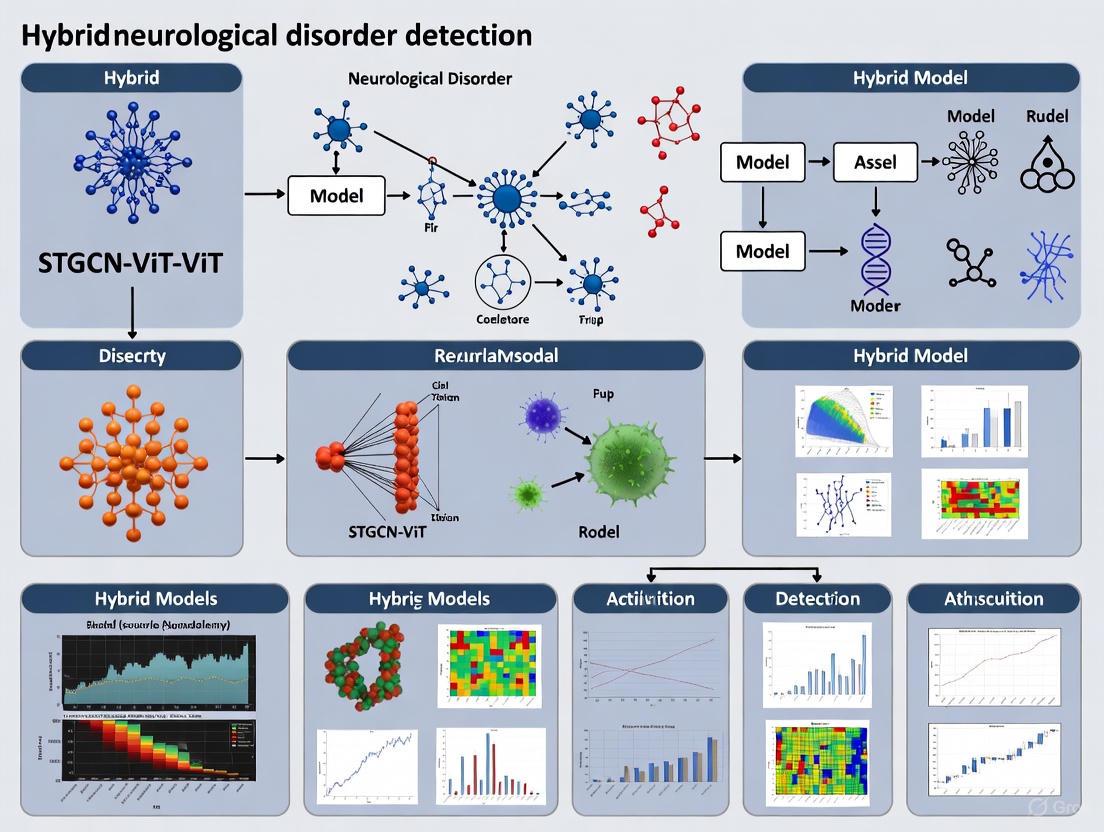
The STGCN-ViT model represents a novel hybrid architecture that integrates convolutional networks, spatial-temporal graph convolutional networks, and vision transformers to address limitations of previous approaches [1]. This integrated framework leverages the strengths of each component: EfficientNet-B0 for spatial feature extraction from high-resolution images, STGCN for modeling temporal dependencies and tracking progression across brain regions, and ViT with self-attention mechanisms to focus on crucial areas and significant spatial patterns in medical scans [1].
The model generates a spatial-temporal graph representing anatomical variations by partitioning spatial features into regions and reducing them, enabling the network to monitor progression across multiple brain areas [1]. This approach addresses a critical limitation of conventional models by explicitly modeling both spatial and temporal dynamics, which is essential for capturing the progressive nature of neurological disorders [1].
Table 2: Performance Comparison of Deep Learning Architectures in Neurological Disorder Detection
| Architecture | Disorder | Dataset | Key Metrics | References |
|---|---|---|---|---|
| STGCN-ViT | Alzheimer's, Brain Tumors | OASIS, HMS | Accuracy: 93.56-94.52%, Precision: 94.41-95.03%, AUC-ROC: 94.63-95.24% [1] | |
| 2D ConvKAN | Parkinson's | PPMI | AUC: 0.973, 97% faster training than conventional CNNs [4] | |
| 3D ConvKAN | Parkinson's | PPMI | AUC: 0.600 (generalization to early-stage cases) [4] | |
| ResNet101-ViT | Alzheimer's | OASIS | Accuracy: 98.7%, Sensitivity: 99.68%, Specificity: 97.78% [2] | |
| Hybrid-RViT | Alzheimer's | OASIS | Training Accuracy: 97%, Testing Accuracy: 95% [5] | |
| ViT-CapsNet | Brain Tumors | BRATS2020 | Accuracy: 90%, Precision: 90%, Recall: 89% [3] | |
| DenseVU-ED | Brain Tumors | BraTS2020 | Segmentation Accuracy: 98.91%, Dice Scores: ET:0.902, WT:0.966 [6] |
Figure 1: Diagnostic challenges and hybrid model solutions. The diagram illustrates how the STGCN-ViT architecture addresses fundamental limitations in neurological disorder diagnosis through integrated spatial-temporal analysis and attention mechanisms.
Experimental Protocols for Hybrid Model Implementation
STGCN-ViT Model Development Protocol
Dataset Preparation and Preprocessing
- Data Sources: Utilize standardized neuroimaging datasets such as OASIS (Open Access Series of Imaging Studies) for Alzheimer's disease research or BRATS2020 for brain tumor studies [1] [3]. Ensure appropriate data use agreements are in place before access [5].
- Image Enhancement: Apply preprocessing filters to improve image quality. Adaptive Median Filters (AMF) effectively reduce noise while preserving edges, and Laplacian filters enhance fine details and tissue boundaries in MRI scans [2].
- Data Augmentation: Address class imbalance through rotation, flipping, and scaling transformations. For neurological disorders with limited early-stage samples, targeted augmentation of underrepresented classes (e.g., mild dementia, early-stage tumors) is crucial [2] [3].
- Volumetric Processing: For 3D MRI data, implement specialized processing pipelines. For Parkinson's disease detection, 3D ConvKAN architectures have demonstrated superior generalization to early-stage cases compared to 2D approaches (AUC 0.600 vs. 0.378) [4].
Model Architecture Configuration
- Spatial Feature Extraction: Implement EfficientNet-B0 as the foundational spatial feature extractor to analyze high-resolution images [1]. Modify standard ResNet or GoogLeNet architectures to reduce computational cost while maintaining feature extraction capabilities [2].
- Temporal Graph Construction: Partition spatial features into regional representations and transform into graph structures where nodes represent brain regions and edges represent anatomical connectivity [1]. STGCN components model these spatial-temporal dependencies to track disease progression across multiple brain regions [1].
- Attention Mechanism Implementation: Configure Vision Transformer components with multi-head self-attention to focus on clinically significant regions [1] [2]. Modify standard ViT architecture to increase attention vertices while managing computational requirements [2].
Model Training and Validation
- Training Protocol: Implement cross-validation with subject-level separation to prevent data leakage. For Parkinson's disease detection, rigorous subject-level evaluation methodologies are essential for assessing generalizability [4].
- Performance Metrics: Evaluate models using comprehensive metrics including accuracy, precision, recall, F1-score, and AUC-ROC [1] [3]. For segmentation tasks, incorporate dice similarity coefficient for tumor subregions [6].
- Interpretability Analysis: Apply Explainable AI (XAI) techniques such as Grad-CAM, SHAP, and LIME to visualize model focus areas and decision processes, enhancing clinical trust and transparency [7] [6].
Cross-Disorder Validation Framework
Multi-Dataset Evaluation
- Within-Dataset Performance: Assess model performance on the same dataset used for training using appropriate cross-validation techniques [4].
- Cross-Dataset Generalizability: Evaluate trained models on independent datasets to test robustness across different imaging protocols and patient populations [4]. For Parkinson's disease detection, models trained on external cohorts (NEUROCON, Tao Wu) should be validated on early-stage PPMI datasets [4].
- Clinical Stage Stratification: Ensure representative inclusion of early-stage cases across all validation sets to properly assess early detection capabilities [4] [2].
Figure 2: STGCN-ViT experimental workflow. The diagram outlines the comprehensive protocol for implementing hybrid models from data preprocessing through multi-stage validation and interpretation.
Essential Research Reagent Solutions
Table 3: Critical Research Resources for Hybrid Model Development
| Resource Category | Specific Examples | Research Application |
|---|---|---|
| Neuroimaging Datasets | OASIS (Alzheimer's), BRATS2020 (Brain Tumors), PPMI (Parkinson's) [1] [4] [3] | Model training, validation, and benchmarking across disorders |
| Preprocessing Tools | Adaptive Median Filters, Laplacian Sharpening Filters [2] | Image quality enhancement, noise reduction, and feature preservation |
| Computational Frameworks | TensorFlow, PyTorch, MONAI | Implementation of hybrid architectures and training pipelines |
| Base Architectures | EfficientNet-B0, ResNet-50/101, Vision Transformers [1] [2] [5] | Foundational components for spatial feature extraction and attention mechanisms |
| Interpretability Tools | Grad-CAM, SHAP, LIME [7] [6] | Model decision visualization and clinical validation |
| Evaluation Metrics | AUC-ROC, Dice Score, Precision, Recall, F1-Score [1] [6] [3] | Comprehensive performance assessment across classification tasks |
The diagnostic challenge in early detection of neurological disorders stems from the complex interplay of subtle anatomical changes, limitations in conventional imaging analysis, and the progressive nature of these conditions. Hybrid deep learning architectures, particularly the STGCN-ViT framework, represent a transformative approach that bridges critical gaps in both spatial and temporal analysis of neuroimaging data. By integrating convolutional networks for spatial feature extraction, graph convolutional networks for modeling temporal dynamics, and vision transformers for global attention mechanisms, these models achieve superior accuracy in classifying Alzheimer's disease, Parkinson's disease, and brain tumors while enabling earlier detection. The experimental protocols and resource frameworks outlined provide researchers with comprehensive methodologies for implementing these advanced architectures, offering promising pathways toward clinically deployable tools that can significantly improve patient outcomes through timely intervention.
Limitations of Conventional MRI Analysis and Human Interpretation in Clinical Practice
Conventional Magnetic Resonance Imaging (MRI) serves as a cornerstone for diagnosing neurological disorders, providing invaluable, non-invasive visualization of brain anatomy. However, its reliance on qualitative, human-centric interpretation presents significant limitations for modern precision medicine and drug development. This application note details the core constraints of conventional MRI analysis, framed within the context of advancing quantitative biomarkers and artificial intelligence (AI), specifically highlighting the rationale for sophisticated models like hybrid Spatial-Temporal Graph Convolutional Networks and Vision Transformers (STGCN-ViT) in neurological research.
Core Limitations of Conventional MRI
The standard paradigm of qualitative MRI analysis is hampered by several intrinsic and operational challenges that affect diagnostic consistency, sensitivity, and quantitative tracking.
Subjectivity and Variability in Human Interpretation
The diagnostic process is inherently vulnerable to human factors, leading to inconsistent interpretations.
- Inter-reader Variability: Different radiologists can arrive at divergent conclusions from the same MRI scan. This subjectivity is particularly critical in early-stage neurological disorders (NDs) like Alzheimer's disease, where subtle anatomical changes are easily missed or interpreted differently [1].
- Lack of Standardized Guidelines: In many areas of MRI, a lack of medical society guidelines with specific imaging parameters means protocols are primarily determined by local expertise and personal preferences. This contributes to wide variability in both image acquisition and interpretation [8].
Qualitative Nature and Arbitrary Units
Conventional MRI provides contrast-weighted images in arbitrary units, limiting their utility as objective biomarkers.
- Non-Quantitative Output: Unlike quantitative MRI (qMRI), which estimates physical tissue parameters (e.g., T1 in ms, ADC in mm²/s), conventional MRI relies on relative signal intensities (T1-weighted, T2-weighted) that are not directly comparable across scanners, sites, or timepoints [9]. This hinders the precise monitoring of disease progression or treatment response essential for clinical trials.
- Focus on Macroscopic Morphology: Conventional structural MRI offers little insight into the underlying microstructure and physiology of the brain, providing measures of regional volume or cortical thickness but failing to detect microscopic changes in tissue integrity that precede gross atrophy [10].
Technical and Operational Challenges
Multiple technical and workflow factors further degrade the consistency and quality of MRI-based diagnosis.
- Artifact Vulnerability: Certain sequences, such as MR cholangiopancreatography and diffusion-weighted imaging (DWI), remain highly vulnerable to artifacts (e.g., motion, susceptibility). Results in clinical practice can be inconsistent, even at sites with a high level of expertise [8].
- Scanner and Protocol Variability: Heterogeneity across scanner vendors, platforms, and imaging protocols (e.g., differences in gradient strengths, slew rates, reconstruction filters) leads to inconsistent outputs, confounding multi-site research and reducing the generalizability of findings [11].
- Workflow Pressures: In clinical environments, competing demands of increasing patient volume and pressure to increase throughput limit the time available for staff to learn and implement new, more advanced techniques, leading to a significant delay in translating methodological advances into practice [8].
Table 1: Key Limitations of Conventional MRI Analysis and Their Impact on Research and Clinical Practice
| Limitation Category | Specific Challenge | Impact on Research & Clinical Practice |
|---|---|---|
| Human Interpretation | Inter-reader variability and subjectivity [1] | Reduces diagnostic reproducibility and agreement in multi-center trials |
| Lack of standardized reporting for artifacts [8] | Hinders systematic quality improvement and issue tracking across sites | |
| Data Characteristics | Qualitative data in arbitrary units [9] | Limits utility as an objective biomarker for tracking subtle changes over time |
| Insensitive to microscopic tissue changes [10] | Unable to detect early pathology before macroscopic structural damage occurs | |
| Technical & Operational | Scanner and protocol variability [11] | Confounds multi-site research findings and limits generalizability |
| High vulnerability to specific artifacts [8] | Compromises diagnostic reliability and can lead to inaccurate interpretations |
Quantitative Evidence and Experimental Validation of Limitations
Empirical data and structured experiments are crucial for quantifying these limitations and validating improved methodologies. The following protocol outlines a approach for benchmarking performance against advanced models.
Experimental Protocol: Benchmarking Diagnostic Accuracy and Robustness
1. Objective: To quantitatively compare the performance of conventional human interpretation against an automated hybrid AI model (STGCN-ViT) in the early detection of neurological disorders from MRI data, assessing accuracy, inter-rater reliability, and robustness to technical variability.
2. Datasets:
- Primary Dataset: Open Access Series of Imaging Studies (OASIS) for Alzheimer's disease applications [1] [12].
- Secondary Dataset: Data from Harvard Medical School (HMS) for general neurological disorder validation [1] [12].
- Inclusion Criteria: T1-weighted, T2-weighted, and FLAIR MRI scans from patients with early-stage NDs and matched healthy controls.
3. Experimental Arms:
- Arm A (Conventional Analysis): A panel of radiologists will independently review conventional MRI scans, providing diagnostic classifications and confidence scores.
- Arm B (AI-Assisted Analysis): The STGCN-ViT model will process the same scans to generate classification outputs [1].
4. Key Performance Metrics:
- Diagnostic Accuracy, Precision, Recall/Sensitivity, Specificity.
- Area Under the Receiver Operating Characteristic Curve (AUC-ROC).
- Inter-rater reliability (Fleiss' Kappa for Arm A).
5. Robustness Analysis: Introduce controlled technical variations (e.g., simulated noise, minor artifacts) to a subset of images and re-evaluate the performance of both arms to assess resilience.
Table 2: Quantitative Comparison of Diagnostic Performance from a Representative Study
| Model / Method | Accuracy (%) | Precision (%) | AUC-ROC Score | Reported Key Advantage |
|---|---|---|---|---|
| Conventional Human Interpretation | Not Explicitly Quantified | Not Explicitly Quantified | Not Applicable | Established clinical standard, provides holistic context |
| Proposed STGCN-ViT Model (Group A) [1] | 93.56 | 94.41 | 94.63 | Integrates spatial-temporal features for early detection |
| Proposed STGCN-ViT Model (Group B) [1] | 94.52 | 95.03 | 95.24 | Superior performance on independent validation dataset |
| Logistic Regression on MRI [1] | 97.00 (for BT) | Not Specified | Not Specified | Demonstrates baseline capability of ML for specific tasks |
| 2D-U-Net + Radiomics [1] | 95.30 | Not Specified | Not Specified | High accuracy in predicting MRI image quality |
The data in Table 2, derived from a study investigating a hybrid STGCN-ViT model, illustrates the potential of advanced AI to achieve high, quantifiable performance metrics that are not consistently reported for conventional human interpretation alone [1]. The integration of spatial feature extraction (via CNN), temporal dynamics (via STGCN), and self-attention mechanisms (via ViT) addresses the inability of conventional methods to capture the complex spatio-temporal progression of neurological diseases [1].
Workflow Comparing Conventional and AI-Driven MRI Analysis
The Scientist's Toolkit: Research Reagent Solutions
Transitioning from qualitative assessment to quantitative, AI-powered analysis requires a suite of specialized tools and resources.
Table 3: Essential Research Materials and Tools for Advanced MRI Analysis
| Item / Resource | Function / Description | Relevance to Model Development |
|---|---|---|
| hMRI Toolbox [10] | Open-source toolbox for generating quantitative parameter maps (R1, R2*, MTSat, PD) from multi-parametric MRI (MPM) data. | Provides standardized input features (qMRI maps) that are more robust than conventional weighted images for model training. |
| FSL (FMRIB Software Library) [10] | A comprehensive library of analysis tools for FMRI, MRI, and DTI brain imaging data. Used for image registration, distortion correction, and diffusion metric calculation (FA, MD). | Critical for pre-processing steps, including aligning dMRI data to MPM space and extracting diffusion-based biomarkers. |
| Multi-parametric MPM Protocol [10] | A protocol using multi-echo 3D FLASH acquisitions to simultaneously capture quantitative R1, R2*, MTSat, and PD maps. | Serves as a source of co-registered, multi-contrast quantitative data that reveals different tissue properties for a holistic view. |
| High-Resolution dMRI Protocol [10] | A diffusion MRI protocol with multiple b=0 acquisitions and many diffusion directions to compute Fractional Anisotropy (FA) and Mean Diffusivity (MD). | Provides microstructural integrity metrics that are complementary to qMRI relaxometry measures, enriching the feature set for models like STGCN. |
| OASIS & ADNI Datasets [1] [12] | Large-scale, open-access neuroimaging databases containing MRI data from patients with Alzheimer's disease and other disorders, alongside healthy controls. | Essential for training and validating AI models on real-world, clinically relevant data, ensuring generalizability. |
| STGCN-ViT Model Architecture [1] [12] | A hybrid deep learning model integrating Convolutional Neural Networks (CNN), Spatial-Temporal Graph Convolutional Networks (STGCN), and Vision Transformers (ViT). | Directly addresses the limitations of conventional analysis by capturing both spatial features and temporal disease dynamics for early diagnosis. |
The field of medical imaging is undergoing a profound transformation, driven by the rapid integration of artificial intelligence (AI) and machine learning (ML) technologies. This evolution marks a significant departure from traditional, often manual interpretation of medical images toward data-driven, automated, and assistive systems that support clinical decision-making at unprecedented levels [13]. The initial adoption of conventional machine learning approaches, which relied heavily on handcrafted feature extraction and traditional classifiers, has progressively given way to sophisticated deep learning architectures capable of learning hierarchical representations directly from raw image data.
This paradigm shift is particularly evident in neurology, where the early diagnosis of neurological disorders (ND) such as Alzheimer's disease (AD) and brain tumors (BT) presents unique challenges due to subtle changes in brain anatomy that can be difficult to detect through human analysis alone [1] [12]. Magnetic Resonance Imaging (MRI) serves as a vital tool for diagnosing and visualizing these disorders, yet standard techniques contingent upon human analysis can be inaccurate, time-consuming, and may miss early-stage symptoms crucial for effective treatment [1]. The integration of ML, particularly deep learning (DL), has opened new avenues for addressing these limitations by providing automated diagnostic systems that deliver accurate findings with minimal margin for error [1].
The emergence of foundation models (FMs) represents the latest frontier in this evolution. These models, trained on broad data using self-supervision at scale, can be adapted to a wide range of downstream tasks, effectively addressing the persistent challenge of labeled data scarcity in medical imaging [14]. This review traces the technological trajectory from traditional models to contemporary deep learning approaches, with particular emphasis on hybrid architectures such as the STGCN-ViT model for neurological disorder detection, while providing detailed application notes and experimental protocols for research implementation.
Evolution of Machine Learning Approaches in Medical Imaging
Traditional Machine Learning Models
Traditional machine learning approaches in medical imaging predominantly relied on handcrafted feature extraction followed by classification using standard algorithms. These methods utilized techniques such as texture analysis, edge detection, and statistical modeling to extract diagnostic patterns from medical images [15]. In neurological applications, features derived from MRI scans—including morphological measurements, texture descriptors, and intensity-based statistics—were fed into classifiers such as Support Vector Machines (SVM), Random Forests, and k-Nearest Neighbors (k-NN) for tasks like Alzheimer's disease classification and brain tumor detection [15].
While these methods were interpretable and aligned with established medical practices, they proved labor-intensive, highly reliant on expert-driven feature engineering, and struggled to generalize across diverse datasets [15]. Their performance was ultimately constrained by the quality and comprehensiveness of the engineered features, which often failed to capture the complex, hierarchical patterns present in medical images.
Deep Learning Revolution
The advent of deep learning, particularly Convolutional Neural Networks (CNNs), transformed medical image analysis by enabling automatic learning of spatial hierarchies directly from raw image data [1] [15]. CNNs demonstrated remarkable capabilities in detecting anomalies and abnormalities within brain imaging studies, making them invaluable tools for diagnosing neurological disorders [1]. Their capacity to learn relevant features automatically from data significantly reduced the dependency on manual feature engineering and consistently outperformed traditional methods across various medical imaging tasks.
More recently, Vision Transformers (ViTs) have emerged as a powerful alternative to CNN-based architectures. By employing self-attention mechanisms, ViTs can concurrently focus on multiple image regions, capturing global contextual information that may be challenging for CNNs with their localized receptive fields [1] [7]. This capability proves particularly valuable for identifying subtle, distributed patterns associated with early-stage neurological disorders.
Hybrid and Foundation Models
The most recent advancements involve the development of hybrid models that combine the strengths of multiple architectures, and foundation models pre-trained on vast, diverse datasets. Hybrid models such as STGCN-ViT integrate spatial feature extraction capabilities of CNNs, temporal modeling of Spatial-Temporal Graph Convolutional Networks (STGCN), and global contextual understanding of Vision Transformers to achieve comprehensive analysis of neurological disorders [1]. Meanwhile, foundation models address the critical challenge of data scarcity in medical imaging by leveraging self-supervised learning on large unlabeled datasets before being fine-tuned for specific clinical tasks with limited annotations [14].
Table 1: Evolution of Machine Learning Approaches in Medical Imaging
| Approach | Key Characteristics | Advantages | Limitations | Representative Applications |
|---|---|---|---|---|
| Traditional ML | Handcrafted features, statistical classifiers | Interpretable, lower computational需求 | Limited representation learning, expert-dependent feature engineering | Brain tumor classification using texture features + SVM |
| Deep Learning (CNNs) | Hierarchical feature learning, convolutional operations | Automatic feature extraction, state-of-the-art performance on many tasks | Large labeled datasets required, limited global context | Alzheimer's detection from MRI, brain tumor segmentation |
| Vision Transformers | Self-attention mechanisms, global context modeling | Superior long-range dependency capture, scalability | Computationally intensive, data-hungry | Whole-slide image analysis, multi-scale medical image classification |
| Hybrid Models | Combined architectures (CNN + ViT + STGCN) | Leverage complementary strengths, spatiotemporal analysis | Implementation complexity, training challenges | STGCN-ViT for neurological disorder progression tracking |
| Foundation Models | Large-scale self-supervised pre-training, task adaptation | Reduced annotation needs, strong generalization | Computational resources, deployment challenges | Multi-institutional medical image analysis across modalities |
The STGCN-ViT Framework for Neurological Disorder Detection
The STGCN-ViT model represents a cutting-edge hybrid framework that strategically integrates convolutional networks, graph neural networks, and transformer architectures to address the complex challenge of neurological disorder detection from medical images. This model specifically addresses critical limitations in existing approaches, including the inadequate capture of long-range dependencies by standard CNNs, the inability to explicitly model temporal progression patterns, and the insufficient integration of both spatial and temporal features in a balanced manner [1].
The architecture employs EfficientNet-B0 for spatial feature extraction from high-resolution medical images, leveraging its proven efficiency and accuracy in visual recognition tasks [1]. The spatial-temporal graph convolutional network (STGCN) component then models temporal dependencies by representing the brain as a graph where nodes correspond to anatomical regions and edges represent structural or functional connectivity, enabling tracking of disease progression across multiple timepoints [1]. Finally, the Vision Transformer (ViT) module incorporates self-attention mechanisms to focus on clinically relevant regions and significant spatial patterns in the scans, providing global contextual understanding [1].
Experimental Protocol for STGCN-ViT Implementation
Materials and Dataset Preparation:
- Datasets: Utilize the Open Access Series of Imaging Studies (OASIS) and Harvard Medical School (HMS) benchmark datasets [1]
- Data Preprocessing: Apply standard neuroimaging preprocessing pipeline including skull stripping, intensity normalization, and spatial registration to a standardized template
- Data Augmentation: Implement random rotations, flipping, intensity variations, and elastic deformations to improve model generalization
- Hardware Requirements: High-performance computing environment with multiple GPUs (NVIDIA A100 or equivalent recommended) for efficient training of deep neural networks
Implementation Protocol:
- Spatial Feature Extraction:
- Initialize EfficientNet-B0 with pre-trained weights
- Process individual MRI slices through the network
- Extract feature maps from intermediate layers
- Apply adaptive pooling to standardize feature dimensions
Spatial-Temporal Graph Construction:
- Parcellate brain images into anatomical regions using standard atlases (AAL, Harvard-Oxford)
- Construct graph nodes from regional features
- Establish edges based on structural connectivity or spatial proximity
- Incorporate temporal dimension by connecting corresponding regions across sequential scans
STGCN Processing:
- Implement graph convolutional layers to capture spatial dependencies
- Apply temporal convolutional layers to model progression patterns
- Utilize skip connections to maintain gradient flow
- Employ batch normalization and dropout for training stability
Vision Transformer Integration:
- Partition STGCN outputs into patches and flatten
- Add positional embeddings and learnable classification token
- Process through multi-head self-attention layers
- Apply multi-layer perceptron head for final classification
Model Training:
- Initialize with Xavier uniform weight initialization
- Use AdamW optimizer with learning rate of 1e-4
- Implement cosine annealing learning rate scheduler
- Employ cross-entropy loss with label smoothing
- Train for 200-300 epochs with early stopping
Model Evaluation:
- Perform k-fold cross-validation (typically 5-fold)
- Evaluate on hold-out test set with balanced class distribution
- Assess using multiple metrics: accuracy, precision, recall, F1-score, and AUC-ROC
STGCN-ViT Architecture Workflow
Performance Analysis and Comparative Evaluation
Quantitative Results of STGCN-ViT Model
The STGCN-ViT model has demonstrated exceptional performance in neurological disorder detection tasks. When evaluated on standard benchmark datasets, the model achieved remarkable metrics that underscore its potential for clinical implementation. On Group A datasets, the approach attained an accuracy of 93.56%, precision of 94.41%, and an Area under the Receiver Operating Characteristic Curve (AUC-ROC) score of 94.63% [1]. For the more challenging Group B datasets, the model attained even better results with an accuracy of 94.52%, precision of 95.03%, and AUC-ROC score of 95.24% [1].
These results significantly outperform both standard and transformer-based models, providing compelling evidence for the model's utility in real-time medical applications and its potential for accurate early-stage neurological disorder diagnosis [1]. The consistency of high performance across different dataset groups further validates the robustness and generalizability of the approach.
Table 2: Performance Comparison of Medical Imaging AI Models
| Model Architecture | Application Domain | Accuracy | Precision | Recall | AUC-ROC | Dataset |
|---|---|---|---|---|---|---|
| STGCN-ViT [1] | Neurological Disorders | 93.56%-94.52% | 94.41%-95.03% | - | 94.63%-95.24% | OASIS, HMS |
| PDSCNN-RRELM [16] | Brain Tumor Classification | 99.22% | 99.35% | 99.30% | - | Brain MRI |
| CNN-ViT Ensemble [7] | Cervical Cancer Diagnosis | 95.10%-99.18% | 95.01%-99.15% | 95.01%-99.18% | - | Mendeley LBC, SIPaKMeD |
| AMRI-Net + EDAL [15] | Multi-modal Integration | 94.95% | - | - | - | ISIC, HAM10000, OCT2017, Brain MRI |
| U-Net Based [13] | Liver Segmentation | - | - | - | - | CT/MRI (HCC) |
| Random Forest [13] | Prostate Cancer Lymph Node Prediction | - | - | - | - | mp-MRI |
Ablation Studies and Component Analysis
Rigorous ablation studies conducted with the STGCN-ViT framework have demonstrated the complementary value of each architectural component. When evaluated independently, the EfficientNet-B0 spatial feature extraction component provided solid baseline performance but lacked temporal understanding crucial for tracking disease progression [1]. The STGCN module alone effectively captured spatiotemporal dynamics but struggled with global contextual relationships in individual scans [1]. The Vision Transformer component excelled at identifying spatially distributed patterns through self-attention mechanisms but lacked explicit temporal modeling capabilities [1].
The integrated framework demonstrated synergistic performance exceeding the arithmetic sum of individual components, validating the architectural hypothesis that spatial, temporal, and global contextual features provide complementary information for neurological disorder diagnosis [1]. This comprehensive approach proved particularly advantageous for early-stage detection where subtle changes across both spatial and temporal dimensions provide the most valuable diagnostic information [1].
Research Reagent Solutions and Computational Tools
Table 3: Essential Research Reagents and Computational Tools
| Resource Category | Specific Tools/Platforms | Function/Purpose | Application in Neurological Disorder Detection |
|---|---|---|---|
| Medical Imaging Datasets | OASIS, HMS, ADNI | Benchmark datasets for model training and validation | Provide standardized MRI data for neurological disorder classification |
| Deep Learning Frameworks | PyTorch, TensorFlow, MONAI | Model implementation, training, and evaluation | Enable development of hybrid architectures like STGCN-ViT |
| Medical Imaging Libraries | NiBabel, DICOM, ITK-SNAP | Medical image reading, processing, and visualization | Handle neuroimaging data format conversion and preprocessing |
| Graph Neural Network Libraries | PyTorch Geometric, DGL | Implementation of graph-based components | Construct and process brain region graphs in STGCN |
| Model Interpretation Tools | SHAP, Grad-CAM, Attention Visualization | Explain model predictions and decision processes | Provide insights into regions of interest in MRI scans |
| Computational Infrastructure | NVIDIA GPUs, Google Colab, AWS | High-performance computing resources | Accelerate training of computationally intensive hybrid models |
| Evaluation Metrics | Scikit-learn, MedPy | Performance assessment and statistical analysis | Quantify classification accuracy, precision, recall, AUC-ROC |
Implementation Protocols for Key Experimental Procedures
Protocol 1: Multi-modal Data Integration and Preprocessing
Objective: To standardize the acquisition and preprocessing of multi-modal medical imaging data for robust model training.
Materials:
- Multi-modal neuroimaging data (T1-weighted, T2-weighted, DTI, fMRI)
- High-performance computing environment with adequate storage
- Medical image processing software (ANTs, FSL, FreeSurfer)
Procedure:
- Data Acquisition and Quality Control
- Acquire structural and functional MRI scans following standardized protocols
- Perform quality assessment using automated tools (MRIQC)
- Exclude datasets with excessive motion artifacts or acquisition errors
Image Preprocessing
- Apply N4 bias field correction for intensity inhomogeneity
- Perform skull stripping using hybrid approach (BET + manual verification)
- Execute spatial normalization to standard template (MNI space)
- Conduct intensity normalization across all scans
Data Augmentation
- Implement geometric transformations (rotation, scaling, elastic deformations)
- Apply intensity-based augmentations (noise injection, contrast adjustment)
- Utilize generative models (GANs) for synthetic data generation if needed
Dataset Partitioning
- Split data into training (70%), validation (15%), and test (15%) sets
- Ensure stratified sampling to maintain class distribution
- Implement cross-validation splits for robust evaluation
Quality Control Measures:
- Visual inspection of preprocessing results
- Quantitative assessment of registration accuracy
- Monitoring of data leakage between splits
Protocol 2: STGCN-ViT Model Training and Optimization
Objective: To establish a standardized protocol for training and optimizing the hybrid STGCN-ViT model.
Materials:
- Preprocessed and partitioned neuroimaging dataset
- Python 3.8+ with deep learning frameworks (PyTorch 1.9+)
- GPU cluster with minimum 16GB VRAM per GPU
Procedure:
- Model Configuration
- Initialize EfficientNet-B0 with ImageNet pre-trained weights
- Configure STGCN with 64-128-256 hidden dimensions
- Set up ViT with 6 attention heads and 512 embedding dimensions
- Implement progressive learning rate warmup
Training Procedure
- Execute mixed-precision training for memory efficiency
- Apply gradient clipping (max norm: 1.0) for training stability
- Implement label smoothing (epsilon: 0.1) for regularization
- Utilize exponential moving average of model weights
Hyperparameter Optimization
- Conduct Bayesian hyperparameter search
- Optimize learning rate (search space: 1e-5 to 1e-3)
- Tune dropout rates (search space: 0.1 to 0.5)
- Optimize batch size (range: 8-32 based on GPU memory)
Regularization Strategies
- Apply stochastic depth (rate: 0.1-0.3)
- Implement weight decay (range: 1e-4 to 1e-2)
- Use data augmentation throughout training
- Employ early stopping with patience of 20 epochs
Validation Framework:
- Monitor training and validation metrics simultaneously
- Perform model selection based on validation AUC-ROC
- Conduct statistical significance testing of results
Experimental Workflow for Medical Imaging AI
Future Directions and Implementation Challenges
Emerging Trends and Research Opportunities
The field of machine learning in medical imaging continues to evolve rapidly, with several promising research directions emerging. Foundation models pre-trained on large-scale, multi-modal medical imaging datasets represent a paradigm shift from task-specific models to general-purpose visual encoders that can be adapted to various downstream applications with minimal fine-tuning [14]. The integration of imaging data with complementary information sources, including clinical records, genomic data, and proteomic profiles, presents opportunities for developing more comprehensive diagnostic and prognostic models [13].
Explainable AI (XAI) techniques are becoming increasingly important for clinical translation, with methods such as SHAP (SHapley Additive exPlanations) and attention visualization providing insights into model decision-making processes [16] [7]. The development of federated learning frameworks addresses critical concerns regarding data privacy and security, enabling multi-institutional collaboration without sharing sensitive patient data [13]. Meanwhile, the emergence of generative AI models offers potential solutions to data scarcity challenges through synthetic data generation and data augmentation [15].
Implementation Challenges and Considerations
Despite the remarkable progress, significant challenges remain in the widespread clinical implementation of ML-based medical imaging systems. Data scarcity and annotation costs continue to constrain model development, particularly for rare neurological disorders [14]. Model generalizability across different scanner types, imaging protocols, and patient populations represents a persistent challenge that requires careful attention to domain adaptation techniques [15].
The computational complexity of hybrid models like STGCN-ViT presents practical deployment challenges in resource-constrained clinical environments [1]. Regulatory approval and standardization processes for AI-based medical devices remain complex and time-consuming, necessitating robust validation across diverse clinical settings [13]. Finally, integration with existing clinical workflows and picture archiving and communication systems (PACS) requires thoughtful interface design and user experience optimization to ensure seamless adoption by healthcare professionals [15].
Addressing these challenges will require collaborative efforts between computer scientists, clinical researchers, regulatory specialists, and healthcare providers to ensure that advanced machine learning technologies can fulfill their potential to revolutionize neurological disorder diagnosis and patient care.
Application Notes: The Spatiotemporal Challenge in Neurology
The Diagnostic Gap in Current Neurological Practice
The progression of neurological disorders (NDs) unfolds across both spatial and temporal dimensions, creating a critical analytical gap in conventional diagnostic approaches. Standard neuroimaging techniques frequently capture static anatomical representations, failing to integrate the dynamic temporal patterns essential for early detection and prognosis. Spatial dynamics refer to the specific brain regions and networks affected by a disease, while temporal dynamics capture the sequence, timing, and evolution of pathological changes. The integration of these dimensions remains a significant challenge in clinical neurology, limiting both diagnostic precision and therapeutic development [1] [17].
Evidence increasingly demonstrates that distinct spatiotemporal progression patterns correlate with specific clinical outcomes across multiple neurological conditions. Research on autoimmune demyelinating diseases has identified discrete atrophy subtypes with unique prognostic implications:
- In Multiple Sclerosis (MS), three spatial atrophy subtypes emerge: cortical (severe cognitive decline), spinal cord (high relapse frequency), and subcortical (severe physical disability) [18] [19]
- In Neuromyelitis Optica Spectrum Disorders (NMOSD), spatial subtypes include cortical (severe cognitive/physical disability), spinal cord (high relapses), and cerebellar (favorable prognosis) [19]
- White Matter Hyperintensity (WMH) progression follows distinct spatiotemporal trajectories: fronto-parietal (delayed onset, more hypertension), radial (widespread progression), and temporo-occipital (more atrial fibrillation) [20]
The clinical impact of these patterns is substantial. For instance, the fronto-parietal WMH subtype shows higher 1-year ischemic stroke recurrence, while the temporo-occipital subtype correlates with worse 3-month outcomes post-stroke [20]. Similarly, advanced stages in MS spinal cord and subcortical atrophy subtypes associate with severe physical disability and cognitive decline [19]. These findings underscore the prognostic value of spatiotemporal analysis for stratified medicine in neurology.
Limitations of Current Analytical Methods
Conventional analytical frameworks face fundamental limitations in capturing the integrated spatiotemporal nature of neurological disease progression:
- Static Imaging Bias: Traditional MRI analysis provides spatial information but typically misses temporal dynamics essential for understanding disease evolution [1]
- Isolated Network Analysis: Most brain network studies examine isolated sequences from sliding windows, failing to capture higher-order spatiotemporal topological patterns [21]
- Temporal Modeling Deficits: Standard Convolutional Neural Networks (CNNs) excel at spatial feature extraction but lack mechanisms for modeling temporal dependencies in disease progression [1]
- Single-Modality Limitations: Approaches relying solely on functional or structural connectivity miss complementary information crucial for comprehensive assessment [21]
These limitations directly impact clinical utility, particularly for early intervention where subtle spatiotemporal signatures often precede overt symptoms. The inability to capture progressive spatial redistribution of pathology over time represents a critical diagnostic gap with implications for drug development and clinical trial design.
Experimental Protocols & Data Presentation
Quantitative Evidence for Spatiotemporal Dynamics
Table 1: Spatiotemporal Subtype Classification in Neurodegenerative and Autoimmune Disorders
| Condition | Spatiotemporal Subtypes | Key Identifying Features | Clinical Correlations |
|---|---|---|---|
| Alzheimer's Disease & MCI [17] | Dynamic Functional Connectivity Patterns | Altered connectivity in hippocampus, amygdala, precuneus, insula | 83.9% accuracy distinguishing AD from healthy controls |
| White Matter Hyperintensities [20] | Fronto-parietal (21%) | Progression from frontal to parietal lobes | Delayed onset, more hypertension, higher 1-year stroke recurrence |
| Radial (46%) | Widespread progression across all lobes | - | |
| Temporo-occipital (33%) | Progression from temporal to occipital lobes | More atrial fibrillation, coronary heart disease, worse 3-month outcomes | |
| Multiple Sclerosis [18] [19] | Cortical | Prominent cortical atrophy | Severe cognitive decline |
| Spinal Cord | Significant cord involvement | High number of relapses | |
| Subcortical | Subcortical gray matter atrophy | Severe physical disability | |
| NMOSD [18] [19] | Cortical | Cortical atrophy patterns | Severe cognitive and physical disability |
| Spinal Cord | Longitudinal extensive cord lesions | High number of relapses | |
| Cerebellar | Cerebellar involvement | Favorable prognosis |
Table 2: Performance Metrics of Advanced Spatiotemporal Analysis Models
| Model/Approach | Disorder | Accuracy | Precision | AUC-ROC | Key Innovation |
|---|---|---|---|---|---|
| STGCN-ViT [1] [12] | General Neurological Disorders | 93.56%-94.52% | 94.41%-95.03% | 94.63%-95.24% | Integrates spatial (CNN), temporal (STGCN), and attention (ViT) mechanisms |
| Dynamic-GRNN [17] | Alzheimer's Disease | 83.9% | - | 83.1% | Combines sliding windows with spatial encoding and dynamic graph pooling |
| Multi-channel Spatio-temporal Graph Attention [21] | Epilepsy & Alzheimer's | Outperforms benchmarks | - | - | Integrates structural and functional connectivity with contrastive learning |
Detailed Experimental Protocols
Protocol 1: STGCN-ViT Model Implementation for Neurological Disorder Classification
Purpose: To implement a hybrid deep learning model that integrates spatial, temporal, and attention mechanisms for early ND detection.
Materials:
- MRI datasets (OASIS, Harvard Medical School)
- Python 3.8+, PyTorch 1.10+
- NVIDIA GPU with ≥12GB VRAM
- Medical image preprocessing tools (ANTs, FSL)
Methodology:
Data Preprocessing
- Convert DICOM to NIfTI format
- Perform skull stripping, intensity normalization, and spatial normalization to MNI space
- Apply data augmentation (rotation, flipping, intensity variations)
Spatial Feature Extraction with EfficientNet-B0
- Utilize pre-trained EfficientNet-B0 backbone for initial spatial feature extraction
- Extract feature maps from convolutional layers at multiple resolutions
- Generate spatial feature tensor of dimensions [B, C, H, W]
Spatio-Temporal Graph Construction
- Partition brain into anatomical regions based on AAL atlas
- Reduce regional features through average pooling
- Construct spatial-temporal graph where nodes represent brain regions and edges represent anatomical connectivity
- Incorporate temporal dimension through sequential scanning
Temporal Dynamics Modeling with STGCN
- Apply spatial-temporal graph convolutional layers
- Model information flow across brain regions using Chebyshev polynomial approximation
- Capture temporal evolution with temporal convolutional layers
- Output temporal feature embeddings
Attention Mechanism with Vision Transformer
- Flatten spatial-temporal features into sequence
- Add positional encodings to preserve spatial information
- Process through multi-head self-attention layers
- Enable model to focus on discriminative spatiotemporal patterns
Classification and Validation
- Final classification through fully connected layers with softmax activation
- Validate using 10-fold cross-validation
- Assess performance using accuracy, precision, recall, F1-score, and AUC-ROC
Validation Metrics: Achieved accuracy of 93.56%-94.52%, precision of 94.41%-95.03%, and AUC-ROC of 94.63%-95.24% on neurological disorder classification tasks [1] [12].
Protocol 2: Dynamic Functional Connectivity Analysis for Alzheimer's Disease
Purpose: To identify early Alzheimer's disease through spatiotemporal analysis of dynamic functional connectivity patterns.
Materials:
- Resting-state fMRI data from ADNI dataset
- Processing pipelines (DPARSF, SPM12)
- Python with NetworkX, PyTorch Geometric
- High-performance computing cluster
Methodology:
fMRI Preprocessing
- Remove first 4 volumes for magnetization equilibrium
- Apply slice timing correction and head motion realignment
- Normalize to MNI space with 3mm isotropic voxels
- Apply temporal filtering (0.01-0.1 Hz) to reduce low-frequency drift
Dynamic Functional Connectivity Construction
- Apply sliding window approach (window size=60-100s, step=1TR)
- Calculate Pearson Correlation Coefficient between brain regions for each window
- Implement Slide Piecewise Aggregation to enhance node features and suppress noise
- Construct dynamic brain network sequence
Graph Neural Network Processing
- Apply spatiotemporal encoding to capture dynamic interactions
- Implement self-attention graph pooling to select key nodes
- Utilize Dynamic Graph Recurrent Neural Network architecture
- Extract spatiotemporal features from dynamic connectivity patterns
Classification and Biomarker Identification
- Train classifier to distinguish Early Mild Cognitive Impairment, AD, and healthy controls
- Identify key affected regions: hippocampus, amygdala, precuneus, insula
- Validate model accuracy through cross-validation
Validation Metrics: Achieved 83.9% accuracy and 83.1% AUC in distinguishing AD from healthy controls [17].
Visualization Framework
STGCN-ViT Model Architecture
Dynamic Functional Connectivity Analysis Workflow
The Scientist's Toolkit: Research Reagent Solutions
Table 3: Essential Research Resources for Spatiotemporal Neurological Analysis
| Resource Category | Specific Tools/Platforms | Primary Function | Application Context |
|---|---|---|---|
| Neuroimaging Datasets | OASIS [1], ADNI [17] [21], UK Biobank [20] | Provide standardized, annotated neuroimaging data for model training and validation | Multi-center studies, algorithm benchmarking, longitudinal analysis |
| Spatiotemporal ML Models | STGCN-ViT [1] [12], Dynamic-GRNN [17], Multi-channel Spatio-temporal Graph Attention [21] | Integrated analysis of spatial and temporal dynamics in brain networks | Early disease detection, progression forecasting, subtype classification |
| Software Libraries | PyTorch Geometric, TensorFlow, EEGlab, SPM12, DPARSF, FreeSurfer | Implement graph neural networks, signal processing, and statistical analysis | Model development, neuroimaging preprocessing, feature extraction |
| Analysis Frameworks | Subtype and Stage Inference (SuStaIn) [18] [20] [19] | Identify distinct spatiotemporal trajectories of disease progression | Disease subtyping, staging, progression modeling |
| Computational Infrastructure | NVIDIA GPUs (≥12GB VRAM), HPC clusters | Accelerate model training and large-scale neuroimaging analysis | Deep learning model training, large dataset processing |
| Multi-modal Integration Tools | Spatial ARP-seq, Spatial CTRP-seq [22] | Simultaneously profile epigenome, transcriptome, and proteome in tissue sections | Molecular mechanism exploration across central dogma layers |
The early diagnosis of neurological disorders (NDs), such as Alzheimer's disease (AD) and Brain Tumors (BT), is highly challenging due to the subtle anatomical changes these conditions cause in the brain. Magnetic Resonance Imaging (MRI) is a vital tool for visualizing these disorders; however, standard diagnostic techniques that rely on human analysis can be inaccurate, time-consuming, and may miss the early-stage symptoms necessary for effective treatment [23] [12]. While Convolutional Neural Networks (CNNs) and other deep learning models have improved spatial feature extraction from medical images, they frequently fail to capture temporal dynamics, which are significant for a comprehensive analysis of disease progression [23].
To address these limitations, a novel hybrid model, the STGCN-ViT, has been developed. This model integrates the strengths of three powerful components: CNNs for spatial feature extraction, Spatial–Temporal Graph Convolutional Networks (STGCN) for capturing temporal dependencies, and Vision Transformers (ViT) with self-attention mechanisms for focusing on crucial spatial patterns [23]. This integration represents a conceptual leap by providing a unified framework that simultaneously models the spatial and temporal evolution of neurological disorders, leading to more accurate and early diagnosis.
Quantitative Performance Analysis
The STGCN-ViT model has been rigorously evaluated on benchmark datasets, including the Open Access Series of Imaging Studies (OASIS) and data from Harvard Medical School (HMS). The model's performance demonstrates its superiority over standard and transformer-based models [23].
Table 1: Performance Metrics of the STGCN-ViT Model on Different Datasets [23]
| Dataset Group | Accuracy (%) | Precision (%) | AUC-ROC Score (%) |
|---|---|---|---|
| Group A | 93.56 | 94.41 | 94.63 |
| Group B | 94.52 | 95.03 | 95.24 |
Table 2: Comparative Analysis of STGCN-ViT Against Other Model Components
| Model or Component | Primary Function | Key Advantage | Application in Neurology |
|---|---|---|---|
| EfficientNet-B0 | Spatial Feature Extraction | Analyzes high-resolution images accurately and efficiently [23]. | Extracts detailed anatomical features from brain MRI scans. |
| Spatial-Temporal GCN (STGCN) | Temporal Feature Extraction | Models progression patterns and dependencies across different brain regions over time [23]. | Tracks the progression of atrophy or lesion development. |
| Vision Transformer (ViT) | Feature Refinement via Self-Attention | Identifies complex, long-range dependencies and subtle patterns in image data [24] [23]. | Highlights critical, distributed biomarkers of early-stage disease. |
| Standard CNN | Spatial Feature Extraction | Effective at recognizing general visual patterns [24]. | Limited by fixed receptive fields and inability to model long-range dependencies [23]. |
Experimental Protocols
Protocol 1: Data Preprocessing and Feature Extraction
This protocol outlines the initial steps for preparing MRI data and extracting foundational features.
- Input Data: Begin with T1-weighted and T2-weighted MRI scans from datasets such as OASIS or HMS [23].
- Spatial Feature Extraction:
- Utilize a pre-trained EfficientNet-B0 model as the foundational feature extractor [23].
- Process the MRI scans through EfficientNet-B0 to generate high-quality spatial feature maps. This step effectively captures detailed anatomical structures.
- Graph Construction:
- Partition the extracted spatial features into distinct regions representing different areas of the brain.
- Construct a spatial-temporal graph where each node corresponds to a brain region. The features of each node are the reduced-dimensionality feature vectors from the CNN.
- The edges between nodes represent the anatomical or functional connections, creating a graph that encapsulates both spatial relationships and the potential for temporal tracking [23].
Protocol 2: STGCN-ViT Model Architecture and Training
This protocol details the core architecture and the procedure for training the hybrid model.
- Temporal Modeling with STGCN:
- Feed the constructed spatial-temporal graph into the STGCN component.
- The STGCN applies graph convolutions to model the temporal dependencies and progression patterns across the sequenced brain region data [23].
- Feature Refinement with Vision Transformer (ViT):
- The output from the STGCN, enriched with spatial-temporal information, is further processed by a Vision Transformer.
- The ViT employs a self-attention mechanism to weigh the importance of different features and regions, focusing on the most discriminative patterns for disease classification [23].
- Model Training and Evaluation:
- Train the integrated STGCN-ViT model using backpropagation and a suitable optimizer (e.g., Adam) with a cross-entropy loss function.
- Evaluate the model on a held-out test set, reporting standard metrics including accuracy, precision, recall, F1-score, and the Area Under the Receiver Operating Characteristic Curve (AUC-ROC) [23].
Model Architecture and Workflow Visualization
Diagram 1: STGCN-ViT Model Workflow
Diagram 2: Logical Relationship: Problem to Solution
The Scientist's Toolkit: Research Reagent Solutions
Table 3: Essential Materials and Computational Tools for STGCN-ViT Research
| Item Name | Function / Description | Specification / Example |
|---|---|---|
| OASIS Dataset | A publicly available neuroimaging dataset providing a large set of MRI data for studying neurological disorders [23]. | Used for training and validating the model for conditions like Alzheimer's disease. |
| Harvard Medical School (HMS) Dataset | A benchmark dataset of brain MRIs, used for evaluating model performance on tasks such as brain tumor detection [23]. | Provides high-quality, annotated medical images. |
| EfficientNet-B0 | A pre-trained CNN backbone for efficient and accurate initial spatial feature extraction from high-resolution MRI scans [23]. | Provides a balance between accuracy and computational efficiency. |
| Spatial-Temporal Graph Convolutional Network (STGCN) | A specialized neural network designed to model data with both spatial and temporal dependencies, crucial for tracking disease progression [23]. | Captures how anatomical changes evolve across the brain over time. |
| Vision Transformer (ViT) | A transformer-based model for image recognition that uses self-attention to identify globally important features for classification [23]. | Excels at capturing long-range dependencies in image data. |
Architecture in Action: Deconstructing the STGCN-ViT Hybrid Model for Medical Imaging
The integration of EfficientNet-B0, Spatio-Temporal Graph Convolutional Networks (STGCN), and Vision Transformer (ViT) represents a sophisticated hybrid approach designed to overcome the limitations of individual deep learning models in analyzing complex medical imaging data. This architecture is particularly impactful in the domain of neurological disorder (ND) detection, where it addresses the critical challenge of capturing both subtle spatial features and their temporal progression in image sequences such as MRI scans. Conventional models often prioritize either spatial or temporal features, but fail to effectively synthesize both, which is essential for identifying early-stage disorders like Alzheimer's disease and brain tumors where anatomical changes are minimal and evolve over time [12] [1]. The proposed hybrid model, termed STGCN-ViT, strategically delegates tasks: EfficientNet-B0 acts as a powerful spatial feature extractor, STGCN models the temporal dynamics and relationships between anatomical regions, and the ViT leverages a self-attention mechanism to focus on the most diagnostically relevant features across the entire image [12] [1]. This synergistic combination has demonstrated superior performance, achieving accuracies over 94% and AUC-ROC scores exceeding 95% on benchmark datasets like OASIS and those from Harvard Medical School, thereby providing a robust tool for real-time clinical applications [12] [1].
Component Fundamentals and Specifications
EfficientNet-B0: The Spatial Feature Extractor
EfficientNet-B0 serves as the foundational spatial feature extractor within the hybrid model. It is the baseline model of the EfficientNet family, which introduced a revolutionary compound scaling method that uniformly scales the network's depth (number of layers), width (number of channels), and input image resolution using a fixed set of coefficients [25] [26]. This principled approach ensures a more efficient balance between model complexity and performance compared to haphazard scaling of single dimensions.
- Architecture and Core Components: The network begins with a stem layer composed of a single 2D convolution with a 3x3 kernel and a stride of 2, followed by batch normalization and a Swish activation function, which provides an initial down-sampling and feature extraction [27]. The body of EfficientNet-B0 is composed of a series of Mobile Inverted Bottleneck Convolution (MBConv) blocks, many of which incorporate Squeeze-and-Excitation (SE) modules to adaptively recalibrate channel-wise feature responses [25] [26]. A key feature of these blocks is depthwise separable convolution, which factorizes a standard convolution into a depthwise convolution (applying a single filter per input channel) and a pointwise convolution (1x1 convolution to combine outputs), drastically reducing computational cost and parameters without significant loss in representational power [25].
- Role in the Hybrid Model: In the STGCN-ViT pipeline, EfficientNet-B0 is responsible for processing individual, high-resolution MRI images. Its primary role is to extract rich, hierarchical, and spatially meaningful features from the brain's anatomy. The model's high efficiency and accuracy, stemming from its compound scaling and MBConv design, make it ideal for this initial processing stage, setting a strong foundation for subsequent temporal and attention-based analysis [12] [1].
Table 1: Detailed Specifications of EfficientNet-B0 Base Network
| Stage | Operator | Resolution | #Channels | #Layers |
|---|---|---|---|---|
| 1 | Conv3x3 | 224x224 | 32 | 1 |
| 2 | MBConv1, k3x3 | 112x112 | 16 | 1 |
| 3 | MBConv6, k3x3 | 112x112 | 24 | 2 |
| 4 | MBConv6, k5x5 | 56x56 | 40 | 2 |
| 5 | MBConv6, k3x3 | 28x28 | 80 | 3 |
| 6 | MBConv6, k5x5 | 14x14 | 112 | 3 |
| 7 | MBConv6, k5x5 | 14x14 | 192 | 4 |
| 8 | MBConv6, k3x3 | 7x7 | 320 | 1 |
| 9 | Conv1x1 & Pooling & FC | 7x7 | 1280 | 1 |
Source: Adapted from [25]
Spatial-Temporal Graph Convolutional Network (STGCN): The Temporal Dynamics Model
The STGCN component is tasked with modeling the temporal dynamics and structural relationships between different brain regions over time. While traditional CNNs are powerful for spatial data, they struggle with non-Euclidean data structures like graphs. STGCN extends Graph Convolutional Networks (GCNs) by performing convolution operations on graph-structured data across both spatial and temporal dimensions [28].
- Core Concepts: The input to the STGCN is a spatio-temporal graph constructed from the features extracted by EfficientNet-B0. In this graph:
- Architecture and Mechanism: The STGCN uses a layered architecture of spatio-temporal graph convolution blocks. Each block typically consists of:
- A spatial graph convolution that aggregates feature information from a node's topological neighbors. This is often implemented using a spectral-based or message-passing approach.
- A temporal convolution (e.g., a 1D convolution with a kernel size of 9) that is applied to the sequence of each node's features, capturing its evolution over time [28]. Skip connections are frequently employed between these blocks to mitigate gradient degradation and allow for the training of deeper networks [28]. This design enables the STGCN to effectively monitor the progression of various brain regions, which is a crucial diagnostic indicator for many neurological disorders [12] [1].
Vision Transformer (ViT): The Attention-Based Feature Refiner
The Vision Transformer (ViT) component introduces a powerful self-attention mechanism to the hybrid model, enabling it to weigh the importance of different features and image patches globally. Originally designed for natural language processing, ViT adapts the transformer architecture for computer vision tasks [29] [30].
- Input Processing and Architecture:
- Patch Embedding: The input image (or feature map) is decomposed into a sequence of fixed-size, non-overlapping patches. Each patch is flattened and linearly projected into an embedding vector [29] [30].
- Positional Encoding: Since the transformer architecture is permutation-invariant, learnable positional encodings are added to the patch embeddings to retain spatial information about the original location of each patch [29].
- Transformer Encoder: The sequence of embedded patches is fed into a standard transformer encoder. The core of this encoder is the multi-head self-attention (MSA) mechanism, which allows the model to simultaneously focus on different patches from the entire sequence and compute their contextual relationships. This is followed by a Multi-Layer Perceptron (MLP) for further processing [30].
- Role in the Hybrid Model: In the STGCN-ViT model, the ViT module is not applied directly to raw images but to the refined spatio-temporal features. Its function is to apply a final, global attention-based feature refinement. By using self-attention, the ViT can identify and focus on the most critical spatial patterns and temporal dependencies identified by the previous components, potentially capturing long-range dependencies that convolutional filters might miss. This leads to a more comprehensive feature set for the final classification of neurological disorders [12] [1].
Table 2: Comparative Analysis of Model Components in Neurological Disorder Detection
| Feature | EfficientNet-B0 | STGCN | Vision Transformer (ViT) |
|---|---|---|---|
| Primary Role | Spatial Feature Extraction | Temporal Dynamics Modeling | Attention-Based Feature Refinement |
| Core Mechanism | MBConv Blocks & Compound Scaling | Spatial-Temporal Graph Convolutions | Multi-Head Self-Attention |
| Input Type | 2D High-Resolution MRI Slices | Spatio-Temporal Graph of Brain Regions | Sequence of Feature Embeddings |
| Output | High-Level Spatial Feature Maps | Temporal Feature Evolution Trajectories | Context-Aware, Weighted Feature Representations |
| Key Advantage | High Accuracy & Computational Efficiency | Models Complex Regional Brain Interactions | Captures Global Context & Long-Range Dependencies |
| Data Requirements | Moderate (Benefits from pre-training) | Requires longitudinal/sequence data | Large datasets for full potential |
Source: Compiled from [12] [25] [29]
Integrated Experimental Protocol for Neurological Disorder Detection
This protocol details the methodology for implementing the hybrid STGCN-ViT model to detect neurological disorders such as Alzheimer's Disease from a series of MRI scans.
Workflow and Signaling Pathway
The following diagram illustrates the logical flow and integration of the three core components within the hybrid model.
Diagram 1: STGCN-ViT Model Workflow for ND Detection. This diagram outlines the sequential processing of medical images, from spatial feature extraction through temporal modeling to final attention-based classification. AD: Alzheimer's Disease; BT: Brain Tumor.
Step-by-Step Procedure
Data Acquisition and Preprocessing
- Datasets: Utilize public benchmark datasets such as the Open Access Series of Imaging Studies (OASIS) or proprietary datasets from institutions like Harvard Medical School (HMS) [12] [1].
- Preprocessing: Standardize all 3D MRI volumes (e.g., T1-weighted). Apply standard pre-processing steps including skull-stripping, intensity normalization, and co-registration to a common template (e.g., MNI space). Data augmentation techniques like random rotation and flipping can be applied to improve model generalization.
Spatial Feature Extraction with EfficientNet-B0
- Input: Individual 2D slices or preprocessed 3D patches from the MRI volumes.
- Protocol: a. Initialize the EfficientNet-B0 model with weights pre-trained on a large-scale dataset like ImageNet. b. Remove the original classification head (global pooling and fully connected layers). c. Process each MRI slice through the network to generate a high-dimensional spatial feature map. d. For each brain scan, aggregate these feature maps to create a comprehensive spatial feature representation [12] [1] [26].
Spatio-Temporal Graph Construction and Modeling
- Graph Construction: a. Node Definition: Parcellate the brain into distinct anatomical regions using an atlas (e.g., AAL). b. Node Features: For each region, reduce the corresponding spatial features from EfficientNet-B0 (e.g., via global average pooling) to form the initial node feature vector. c. Edge Definition: Construct an adjacency matrix defining the connections between nodes. This can be based on structural connectivity (from DTI), functional connectivity, or simply anatomical proximity [12] [1] [28].
- STGCN Processing: a. Build a spatio-temporal sequence by linking graph snapshots from consecutive patient visits. b. Feed this sequence into the STGCN model. c. The STGCN performs graph convolutions spatially and 1D convolutions temporally, outputting a refined feature representation that encapsulates the temporal evolution of each brain region [12] [28].
Attention-Based Feature Refinement with ViT
- Input Preparation: The output features from the STGCN are serialized into a sequence of embeddings. If necessary, a learnable
[CLS]token is prepended to the sequence [30]. - ViT Processing:
a. Add positional encodings to the sequence to retain order information.
b. Process the sequence through multiple transformer encoder layers, each employing multi-head self-attention.
c. The output corresponding to the
[CLS]token (or the averaged output of all tokens) is used as the final, context-aware representation of the patient's brain scan sequence for classification [12] [1] [30].
- Input Preparation: The output features from the STGCN are serialized into a sequence of embeddings. If necessary, a learnable
Model Output and Evaluation
- Classification Head: The final feature vector from the ViT is passed through a fully connected layer with a softmax activation function to generate probability scores for each diagnostic class (e.g., Healthy, Alzheimer's Disease, Brain Tumor) [12].
- Evaluation Metrics: Validate the model on a held-out test set. Report standard performance metrics including Accuracy, Precision, Recall, F1-Score, and the Area Under the Receiver Operating Characteristic Curve (AUC-ROC). The model should be compared against standard and transformer-based baseline models [12] [1].
The Scientist's Toolkit: Research Reagent Solutions
Table 3: Essential Computational Reagents for STGCN-ViT Research
| Research Reagent | Function & Specification | Example/Tool |
|---|---|---|
| Benchmark Neuroimaging Datasets | Provides standardized, annotated data for training and validation. Must contain longitudinal MRI data. | OASIS, ADNI, Harvard Medical School (HMS) datasets [12] [1] |
| Computational Framework | Software environment for building, training, and evaluating complex deep learning models. | PyTorch, TensorFlow, Keras with specialized libraries for GNNs (e.g., PyTorch Geometric) |
| Anatomical Brain Atlas | Digital template for parcellating the brain into distinct regions of interest (Nodes for STGCN). | Automated Anatomical Labeling (AAL) Atlas, Harvard-Oxford Atlas |
| Graph Construction Tool | Utility to define spatial relationships (edges) between brain regions for building the graph input for STGCN. | Custom scripts based on DTI tractography or anatomical proximity matrices [28] |
| Pre-trained EfficientNet-B0 Weights | Provides a robust initialization for the spatial feature extractor, significantly improving convergence and performance. | Weights from ImageNet or specialized medical imaging competitions |
Within the framework of developing hybrid STGCN-ViT (Spatial-Temporal Graph Convolutional Network - Vision Transformer) models for neurological disorder detection, the initial step of robust spatial feature extraction from high-resolution brain anatomy is paramount. This phase is critical for converting complex anatomical patterns in medical images into structured, discriminative data representations that subsequent model components can process. The EfficientNet-B0 architecture has emerged as a superior foundation for this task, offering a balanced trade-off between computational efficiency and high representational power. Its application allows researchers to capture intricate spatial features from brain scans, forming the essential input for temporal dynamics analysis by STGCN and global relationship modeling by ViT components. This document outlines detailed protocols and application notes for implementing EfficientNet-B0 in brain imaging pipelines, specifically tailored for neurological disorder research contexts where early detection of conditions like Alzheimer's disease and brain tumors depends on identifying subtle anatomical alterations.
Quantitative Model Specifications
Table 1: EfficientNet-B0 Architectural and Performance Specifications
| Parameter Category | Specification Details | Research Implications |
|---|---|---|
| Top-1 Accuracy (ImageNet-1K) | 77.692% [31] | Demonstrates strong baseline feature extraction capability for transfer learning |
| Top-5 Accuracy (ImageNet-1K) | 93.532% [31] | High confidence in top predictions increases feature reliability |
| Parameter Count | 5,288,548 [31] | Enables deployment in compute-limited environments without sacrificing performance |
| Computational Requirement | 0.39 GFLOPS [31] | Facilitates processing of high-volume medical imaging datasets |
| Default Input Resolution | 224x224 pixels [32] | Standardized input size for consistent feature extraction pipelines |
| Core Innovation | Compound model scaling [32] | Balanced scaling of network depth, width, and resolution optimizes feature learning |
Experimental Protocols
Protocol: Integration of EfficientNet-B0 within STGCN-ViT Framework
Objective: To extract discriminative spatial features from brain MRI scans using EfficientNet-B0 for subsequent processing by STGCN and ViT modules in a hybrid neurological disorder detection pipeline.
Background: In the STGCN-ViT model, EfficientNet-B0 serves as the primary spatial feature extractor, converting raw MRI inputs into structured feature representations that encapsulate critical neuroanatomical information. These features are then structured into region-based graphs for temporal analysis by STGCN and further refined through attention mechanisms in the ViT component [12] [1].
Materials:
- Brain MRI Datasets: OASIS (Open Access Series of Imaging Studies) and Harvard Medical School (HMS) benchmark datasets [12]
- Software Framework: PyTorch with torchvision models interface [31]
- Preprocessing Tools: Image normalization and resizing utilities compatible with EfficientNet-B0 requirements
Procedure:
- Input Preprocessing:
- Resize input MRI scans to 256x256 pixels using bicubic interpolation
- Perform central crop to 224x224 pixels to match EfficientNet-B0 input expectations
- Rescale pixel values to [0.0, 1.0] range
- Apply normalization using mean=[0.485, 0.456, 0.406] and std=[0.229, 0.224, 0.225] [31]
Feature Extraction:
- Initialize EfficientNet-B0 with ImageNet-pretrained weights
- Remove the final classification layer to access the feature space
- Process preprocessed MRI volumes through the network to generate high-dimensional feature maps
- These features capture hierarchical spatial patterns from basic edges to complex neuroanatomical structures
Feature Transformation for STGCN:
- Partition the extracted spatial features into region-based representations
- Construct spatial-temporal graphs where nodes represent brain regions and edges encode anatomical connectivity
- Reduce feature dimensionality as needed to optimize computational efficiency while preserving discriminative information [12]
Output Integration:
- Feed the structured spatial features to the STGCN component for temporal dynamics modeling
- The ViT component subsequently applies self-attention mechanisms to focus on clinically relevant regions [1]
- The complete pipeline enables comprehensive analysis of both spatial and temporal patterns in neurological disorder progression
Validation:
- Expected performance benchmarks: 93.56% accuracy (Group A) and 94.52% accuracy (Group B) on neurological disorder classification tasks [12]
- Comparative analysis against standard and transformer-based models to verify performance improvement
Protocol: Transfer Learning for Domain Adaptation
Objective: To adapt ImageNet-pretrained EfficientNet-B0 weights for optimal performance on brain MRI analysis through targeted fine-tuning.
Procedure:
- Model Initialization:
- Load EfficientNet-B0 with pretrained ImageNet-1K weights using PyTorch framework [31]
- Replace the final fully connected layer with a task-specific head matching the target neurological disorder classification categories
Progressive Fine-Tuning:
- Initially freeze all layers except the final classification head and train for 5-10 epochs
- Gradually unfreeze intermediate layers while monitoring validation performance
- Employ differential learning rates, with lower rates for earlier layers and higher rates for later layers
Regularization Strategy:
- Implement strong data augmentation (random rotations, flips, intensity variations) to prevent overfitting
- Utilize dropout and weight decay appropriate for medical imaging data characteristics
- Apply early stopping based on validation loss plateau
Workflow Visualization
Spatial Feature Extraction Pipeline for STGCN-ViT Model
The Scientist's Toolkit
Table 2: Essential Research Reagents and Computational Resources
| Resource Category | Specific Tool/Platform | Function in Research Pipeline |
|---|---|---|
| Deep Learning Framework | PyTorch with torchvision [31] | Provides EfficientNet-B0 implementation and pretrained weights for rapid prototyping |
| Neuroimaging Data | OASIS, Harvard Medical School datasets [12] | Benchmark datasets for model training and validation with clinical ground truth |
| Brain Atlas | NextBrain AI-assisted atlas [33] [34] | Enables precise region identification and segmentation for spatial-temporal graph construction |
| Model Architectures | EfficientNet-B0, STGCN, Vision Transformer [12] [1] | Core components of the hybrid model for comprehensive spatial-temporal analysis |
| Computational Hardware | GPU-accelerated workstations | Necessary for processing high-resolution 3D MRI volumes within feasible timeframes |
| Evaluation Metrics | Accuracy, Precision, AUC-ROC [12] | Standardized performance measures for model validation and comparison |
Analytical Framework for Feature Interpretation
Table 3: Multi-scale Feature Representation in Brain MRI Analysis
| Feature Hierarchy Level | Anatomical Correlates in Brain MRI | Clinical Relevance for Neurological Disorders |
|---|---|---|
| Shallow Features (Early Layers) | Basic edges, textures, intensity gradients [12] | Detection of gross anatomical boundaries, tissue type differentiation |
| Intermediate Features (Middle Layers) | Complex shape primitives, regional patterns | Identification of structural changes in specific brain regions |
| Deep Features (Later Layers) | High-level anatomical constructs, structural relationships [1] | Detection of subtle pathological markers indicative of early disease stages |
| Spatial-Temporal Features (STGCN) | Progressive anatomical changes across timepoints [12] | Tracking disease progression, monitoring treatment efficacy |
| Attention-Weighted Features (ViT) | Clinically significant regions with discriminative power [1] | Focus on disease-specific vulnerable areas for improved diagnostic specificity |
Validation Framework and Performance Benchmarking
Objective: To establish standardized evaluation protocols for assessing the efficacy of EfficientNet-B0 derived features in neurological disorder classification tasks.
Procedure:
- Dataset Stratification:
- Implement k-fold cross-validation (typically k=5) to ensure robust performance estimation
- Maintain strict separation between training, validation, and test sets to prevent data leakage
- Ensure balanced representation of disease stages and demographic factors across splits
Performance Metrics:
- Track accuracy, precision, recall, and F1-score for classification performance
- Calculate AUC-ROC to evaluate model discrimination capability across sensitivity thresholds [12]
- Compare against baseline models (standard CNNs, transformer-only architectures) to establish performance improvement
Clinical Correlation:
- Validate feature importance against known neuroanatomical vulnerability patterns in target disorders
- Conduct ablation studies to quantify contribution of individual model components to overall performance
- Perform statistical significance testing to ensure observed improvements are not due to random variation
Expected Outcomes:
- The integrated STGCN-ViT model with EfficientNet-B0 feature extraction should achieve approximately 94% accuracy in neurological disorder classification [12]
- Significant improvement in early detection capability compared to conventional approaches, with precision metrics exceeding 95% [1]
- Demonstrated robustness across diverse patient populations and imaging protocols
The integration of temporal dynamics into disease progression models represents a frontier in computational neurology. While conventional deep learning models excel at spatial feature extraction from medical images, they often fail to capture the temporal patterns essential for understanding neurodegenerative diseases. Spatio-Temporal Graph Convolutional Networks (STGCN) address this limitation by modeling both spatial relationships and their evolution over time, providing a powerful framework for quantifying disease trajectories. When integrated with Vision Transformers (ViT) in hybrid architectures, these models enable unprecedented precision in early detection and staging of neurological disorders, offering potentially transformative applications in clinical trial enrichment and therapeutic development.
STGCN Fundamentals in Neurological Context
Spatio-Temporal Graph Convolutional Networks extend graph convolutional operations to capture dynamic patterns in data with inherent structural relationships. In neurological applications, STGCNs represent brain regions as nodes in a graph, with edges representing anatomical or functional connections. The temporal dimension captures how these regional interactions evolve throughout disease progression.
The fundamental innovation of STGCN lies in its ability to independently extract spatial and temporal features, significantly reducing information loss that occurs when these dimensions are processed jointly [35]. This independent processing ensures extraction of useful features regardless of exact spatial and temporal points, making it particularly suitable for modeling the heterogeneous progression patterns observed in neurological disorders.
STGCN architectures typically employ spatial graph convolutional layers that operate on brain region connectivity patterns, coupled with temporal convolutional layers that model progression dynamics. This dual approach has demonstrated computational efficiency while maintaining high accuracy, enabling deployment in resource-constrained environments including potential edge computing applications in clinical settings [35].
Performance Benchmarks: STGCN in Neurological Disorder Detection
Alzheimer's Disease Detection Performance
Table 1: STGCN Performance in Alzheimer's Disease Classification
| Model Architecture | Dataset | Accuracy | AUC-ROC | Key Biomarkers |
|---|---|---|---|---|
| STGCN-ViT (Proposed) | OASIS | 93.56% | 94.63% | Structural MRI, Cognitive scores |
| STGCN-ViT (Proposed) | HMS | 94.52% | 95.24% | Multi-modal biomarkers |
| Dynamic-GRNN | ADNI | 83.9% | 83.1% | Functional connectivity, Hippocampal volume |
The STGCN-ViT hybrid model demonstrates exceptional performance in Alzheimer's disease classification, achieving up to 94.52% accuracy and 95.24% AUC-ROC on benchmark datasets [1]. This represents significant improvement over conventional approaches, particularly in early-stage detection where subtle spatial and temporal changes must be captured simultaneously.
In practical applications, STGCN models have successfully identified key affected regions in Alzheimer's progression, including the left hippocampus, right amygdala, and left inferior parietal lobe - areas known to be associated with memory function and early Alzheimer's pathology [17]. This spatial localization capability combined with temporal tracking provides unprecedented insight into disease progression patterns.
Cross-Discipline Application Performance
Table 2: STGCN Performance Across Disease Domains
| Application Domain | Data Modality | Performance | Temporal Resolution |
|---|---|---|---|
| Neurological Disorders | MRI | 94.52% accuracy | Longitudinal scans (months-years) |
| Human Action Recognition | Skeleton data | 92.2% accuracy | Real-time (ms-s) |
| Infectious Disease Forecasting | Epidemiological data | 12-week prediction | Weekly incidence data |
The versatility of STGCN architectures is evidenced by their application across diverse medical domains. In human action recognition for healthcare monitoring, STGCN models achieved 92.2% accuracy on skeleton datasets using only joint data and fewer parameters [35]. This efficiency demonstrates the model's suitability for real-time patient monitoring applications where computational resources may be limited.
For infectious disease prediction, STGCNs have successfully incorporated spatial factors from surrounding cities with historical incidence data to predict Hand, Foot and Mouth Disease outbreaks with 12-week forecasting capability at the prefecture level [36]. This cross-disciplinary success underscores the generalizability of the STGCN approach for spatio-temporal modeling in healthcare.
Experimental Protocols for STGCN Implementation
STGCN-ViT Hybrid Model Protocol
Data Preparation and Preprocessing
- Imaging Data: Collect T1-weighted and T2-weighted MRI scans from standardized datasets (OASIS, ADNI, HMS)
- Spatial Normalization: Register all images to standard template (MNI space) using linear and non-linear transformations
- Graph Construction: Define nodes based on anatomical atlas (AAL, Desikan-Killiany); edges based on structural connectivity or spatial proximity
- Temporal Alignment: For longitudinal data, align scans by clinical onset or diagnosis date
- Data Augmentation: Apply random rotations, flipping, and intensity variations to improve model generalization
Model Architecture Specification
- Spectral Feature Extraction: Implement EfficientNet-B0 for initial spatial feature extraction from MRI slices
- Graph Construction: Convert extracted features to graph structure with region-based nodes
- STGCN Configuration:
- Spatial Graph Convolution: Chebyshev polynomial approximation with K=3
- Temporal Convolution: 1D convolutional layers with kernel size 9
- Activation: PreLU with batch normalization
- Dropout rate: 0.5 for regularization
- ViT Integration:
- Patch size: 16×16
- Attention heads: 12
- Hidden size: 768
- Transformer layers: 12
Training Protocol
- Optimization: Adam optimizer with initial learning rate 0.001, reduced by factor 0.1 after 10 epochs of no improvement
- Loss Function: Weighted cross-entropy to handle class imbalance
- Batch Size: 16 due to memory constraints with 3D data
- Validation: 5-fold cross-validation with strict separation of patients across folds
- Regularization: Early stopping with patience of 15 epochs monitoring validation loss
Evaluation Metrics
- Primary: Accuracy, Precision, Recall, F1-score, AUC-ROC
- Secondary: Specificity, Sensitivity, Balanced Accuracy
- Statistical: Confidence intervals via bootstrapping, p-values for model comparison
Dynamic Functional Connectivity Analysis Protocol
fMRI Preprocessing Pipeline
- Software: SPM12, FSL, or AFNI for standard preprocessing
- Steps: Slice timing correction, realignment, normalization, smoothing (6mm FWHM)
- Quality Control: Frame-wise displacement <0.5mm, visual inspection of artifacts
- Denoising: Regression of white matter, CSF signals, and motion parameters
Dynamic Brain Network Construction
- Sliding Window: Window length=30 volumes, step size=1 volume
- Connectivity Metric: Pearson correlation coefficient between regional time series
- Graph Definition: Nodes=predefined atlas regions, edges=correlation values
- Feature Enhancement: Apply Slide Piecewise Aggregation (SPA) to enhance temporal expression
Dynamic-GRNN Implementation
- Spatio-temporal Encoding: Joint modeling of brain network functionality and time series dynamics
- Graph Pooling: Temporal SAGPooling to select Top-K nodes based on cross-temporal attention weights
- Core Node Identification: Calculate degree centrality, betweenness centrality, and closeness centrality
- Classification: Fully connected layers with softmax output for patient stratification
Architectural Visualization
STGCN-ViT Hybrid Model Workflow
STGCN-ViT Hybrid Model Architecture
Temporal Dynamics Modeling in Disease Progression
Temporal Dynamics in Disease Progression
Research Reagent Solutions
Table 3: Essential Research Resources for STGCN Implementation
| Resource Category | Specific Resource | Application Purpose | Key Features |
|---|---|---|---|
| Neuroimaging Datasets | OASIS | Model training/validation | Longitudinal MRI, multi-age span, clinical dementia ratings |
| ADNI | Alzheimer's progression modeling | Multi-modal data (MRI, PET, genetic, cognitive) | |
| TRACK-HD | Huntington's disease progression | Motor, cognitive, MRI biomarkers in premanifest HD | |
| Computational Frameworks | PyTorch Geometric | Graph neural network implementation | Specialized GCN layers, benchmark datasets |
| TensorFlow/Keras | Deep learning model development | High-level API, multi-GPU support | |
| Nilearn | Neuroimaging data manipulation | Brain graph construction, connectivity analysis | |
| Biomarker Analysis Tools | SPM12 | fMRI/MRI preprocessing | Statistical parametric mapping, normalization |
| FSL | Brain extraction, registration | FMRIB Software Library, diffusion processing | |
| FreeSurfer | Cortical reconstruction | Automated segmentation, surface-based analysis | |
| Evaluation Metrics | scikit-learn | Model performance assessment | Classification metrics, statistical testing |
| NeuroKit2 | Physiological signal analysis | Signal processing, feature extraction |
Clinical Translation and Applications
Clinical Trial Enrichment
The STGCN-ViT framework demonstrates particular promise in clinical trial enrichment, a critical challenge in neurodegenerative drug development. By accurately staging patients and estimating progression risk, these models can identify individuals most likely to progress during trial periods, significantly reducing required cohort sizes. The Temporal Event-Based Model (TEBM) has shown potential to achieve 80% power with less than half the cohort size compared to random selection [37], addressing a major barrier in trial economics.
For preventative clinical trials targeting pre-clinical individuals, STGCN models enable dichotomization of slow early-stage and fast early-stage progressors, creating opportunities for interventions when treatments are likely most effective. This stratification capability is particularly valuable in conditions like Alzheimer's where pathological changes begin years before clinical symptoms manifest.
Personalized Progression Forecasting
Beyond population-level modeling, STGCN architectures support individualized progression forecasting by integrating patient-specific biomarker data with learned spatio-temporal patterns. The Dynamic-GRNN approach identifies key affected regions such as the left hippocampus, right amygdala, and left inferior parietal lobe [17], providing clinicians with specific anatomical targets for monitoring and intervention.
The probabilistic nature of the TEBM framework generates confidence intervals around progression estimates, enabling transparent communication of forecast uncertainty in clinical decision-making. This temporal precision facilitates personalized monitoring schedules and informs optimal timing for therapeutic interventions based on individual progression trajectories rather than population averages.
The integration of STGCN models within hybrid STGCN-ViT architectures represents a paradigm shift in modeling neurological disease progression. By capturing both spatial relationships and their temporal evolution, these approaches overcome critical limitations of conventional deep learning models that treat spatial and temporal dimensions separately. The resulting performance improvements in early detection, patient stratification, and progression forecasting demonstrate the transformative potential of spatio-temporal modeling in neurology.
As neurological disorders increasingly constitute a global health crisis, the ability to precisely quantify disease timelines and individual progression patterns becomes essential for developing effective therapeutic strategies. STGCN-based frameworks provide the analytical foundation for this precision neurology approach, creating opportunities for earlier intervention, optimized clinical trials, and ultimately improved patient outcomes across the spectrum of neurodegenerative diseases.
The integration of self-attention mechanisms within Vision Transformer (ViT) architectures has revolutionized the analysis of medical images, enabling data-driven identification of disease-critical brain regions without heavy reliance on prior anatomical assumptions. Within the broader scope of hybrid Spatio-Temporal Graph Convolutional Network-Vision Transformer (STGCN-ViT) models for neurological disorder detection, the capability to pinpoint diagnostically relevant regions provides a critical foundation for both spatial feature extraction and temporal progression tracking. This approach aligns with the core objective of developing interpretable artificial intelligence for clinical applications, where understanding model decision-making is as crucial as diagnostic accuracy itself. By leveraging the self-attention mechanism's ability to weigh the importance of different image patches, ViT-based models can automatically discover and focus on regions exhibiting pathological alterations, thereby uncovering meaningful biomarkers directly from data.
The application of this paradigm spans numerous neurological conditions, including Alzheimer's disease (AD), Parkinson's disease (PD), Attention-Deficit/Hyperactivity Disorder (ADHD), and movement disorders, demonstrating the versatility of the approach across different neuroimaging modalities and disease pathologies. This document provides comprehensive application notes and experimental protocols for implementing these methodologies, with particular emphasis on their integration within hybrid STGCN-ViT frameworks for superior neurological disorder detection and characterization.
Self-Attention in ViT for Regional Analysis
The self-attention mechanism in Vision Transformers processes input images by dividing them into patches, projecting them into embeddings, and computing relationships between all patches regardless of spatial distance. This global receptive field enables the model to capture long-range dependencies between distributed brain regions that often exhibit coordinated pathological changes in neurological disorders. The multi-head self-attention mechanism computes attention weights between all patch pairs, creating an attention map that highlights regions with significant influence on the final classification decision.
When integrated into hybrid STGCN-ViT models, the self-attention component specifically addresses the spatial analysis dimension, identifying critical diagnostic regions that subsequently inform temporal modeling through graph convolutional networks. This division of labor leverages the complementary strengths of both architectures: ViT's superior spatial contextualization and STGCN's capacity for modeling progressive pathological changes across time-series data. The regional importance scores derived from attention maps can directly inform the construction of node features and connectivity weights in the spatial-temporal graph component, creating a cohesive analytical pipeline.
Case Studies and Performance Evaluation
Regional Attention-Enhanced ViT for Alzheimer's Disease
The Regional Attention-Enhanced Vision Transformer (RAE-ViT) represents a specialized implementation explicitly designed to prioritize disease-critical brain regions in Alzheimer's diagnosis using structural MRI (sMRI) data. The framework incorporates a regional attention module (RAM) that selectively weights features from regions with known pathological significance, hierarchical self-attention to capture both local and global brain patterns, and multi-scale feature extraction [38] [39].
In comprehensive evaluations using the Alzheimer's Disease Neuroimaging Initiative (ADNI) dataset comprising 1152 sMRI scans, RAE-ViT demonstrated state-of-the-art performance in distinguishing between Alzheimer's disease (AD), Mild Cognitive Impairment (MCI), and Normal Control (NC) subjects, achieving an accuracy of 94.2%, sensitivity of 91.8%, specificity of 95.7%, and AUC of 0.96 [38]. The model significantly outperformed standard ViT (89.5% accuracy) and CNN-based approaches like ResNet-50 (87.8% accuracy), validating the efficacy of its enhanced attention mechanism [39].
Table 1: Performance Comparison of Alzheimer's Disease Classification Models
| Model | Accuracy | Sensitivity | Specificity | AUC | Dataset |
|---|---|---|---|---|---|
| RAE-ViT | 94.2% | 91.8% | 95.7% | 0.96 | ADNI (1152 scans) |
| Standard ViT | 89.5% | - | - | - | ADNI |
| ResNet-50 | 87.8% | - | - | - | ADNI |
| Hybrid STGCN-ViT | 93.56% | - | - | 94.63% | OASIS, HMS |
| ViT (Meta-Analysis) | 92.5%* | 92.5% | 95.7% | 0.924 | Multiple datasets |
*Sensitivity value from meta-analysis [40]
A key advantage of the RAE-ViT framework is its interpretability; the generated attention maps closely align with clinically established AD biomarkers, demonstrating high spatial overlap with hippocampal regions (Dice coefficient: 0.89) and ventricular areas (Dice coefficient: 0.85) [38] [39]. This alignment with known pathology builds clinical trust and provides validation of the model's decision-making process. The framework also exhibited robust performance across scanner variations (92.5% accuracy on 1.5T scans) and under noise conditions (92.5% accuracy with 10% Gaussian noise), supporting its potential clinical applicability [39].
Transformer-Based Structural Connectivity Networks for ADHD
The application of transformer-based models extends to ADHD diagnosis, where structural connectivity networks (SCNs) built from MRI data have revealed altered connectivity patterns associated with the disorder. Using a transformer encoder architecture applied to the ADHD-200 dataset (947 individuals across 8 centers), researchers constructed SCNs that quantified the strength of connectivity between different brain regions [41].
The model achieved a diagnostic accuracy of 71.9% with an AUC of 0.74, identifying significant connectivity alterations in regions responsible for motor and executive function [41]. Statistical analysis revealed significant between-group differences in connectivity patterns (paired t-test: P = 0.81 × 10⁻⁶), particularly highlighting the importance of the thalamus and caudate, which showed markedly different importance rankings between ADHD and control groups [41].
Table 2: Regional Importance in Neurological Disorder Classification
| Disorder | High-Attention Brain Regions | Clinical Correlation |
|---|---|---|
| Alzheimer's Disease | Hippocampus, Ventricles, Entorhinal Cortex | Memory processing, brain volume changes |
| ADHD | Thalamus, Caudate, Lingual Gyrus, Precuneus Lobe | Motor control, executive function, visual processing |
| Parkinson's Disease | Prefrontal Cortex, Frontal Polar Cortex | Motor control, cognitive functions |
This approach demonstrates how transformer self-attention mechanisms can automatically derive connectomic relationships from structural MRI data without predefined network architectures, offering an objective, data-driven method for identifying neurobiological markers in ADHD.
Hybrid STGCN-ViT for Neurological Disorders
The hybrid STGCN-ViT model represents a comprehensive framework that integrates convolutional neural networks (CNN), Spatial-Temporal Graph Convolutional Networks (STGCN), and Vision Transformer (ViT) components to address both spatial and temporal dynamics in neurological disorder progression [1] [12]. In this architecture, EfficientNet-B0 performs initial spatial feature extraction, STGCN models temporal dependencies, and ViT applies attention mechanisms for feature refinement and regional importance weighting.
When evaluated on the Open Access Series of Imaging Studies (OASIS) and Harvard Medical School (HMS) datasets for neurological disorder classification, the hybrid model achieved competitive performance with 93.56% accuracy, 94.41% precision, and an AUC-ROC score of 94.63% in Group A, and 94.52% accuracy, 95.03% precision, and 95.24% AUC-ROC in Group B [1] [12]. This performance advantage over standard and transformer-based models highlights the benefit of integrating spatial and temporal analysis capabilities within a unified framework.
Experimental Protocols
Regional Attention-Enhanced ViT Implementation Protocol
Objective: Implement RAE-ViT for Alzheimer's disease classification using structural MRI data with interpretable regional attention mapping.
Dataset Preparation:
- Utilize the ADNI dataset or comparable sMRI data collection
- Apply standard preprocessing: skull stripping, normalization, and registration to common template (e.g., MNI space)
- Partition data into training, validation, and test sets (typical ratio: 70:15:15)
- Implement data augmentation: random rotations, flipping, intensity variations
Model Architecture Specifications:
- Patch embedding: Divide 3D sMRI volumes into 16×16×16 patches with overlap
- Regional Attention Module (RAM): Implement learnable attention weights for predefined brain regions
- Hierarchical self-attention: Multi-head attention with 12 heads and 768 hidden dimensions
- Multi-scale feature extraction: Process patches at multiple resolutions (1×, 0.5×, 0.25× original scale)
- Classification head: 3-layer MLP with softmax output for AD/MCI/NC classification
Training Procedure:
- Pretraining: Initialize with weights from CheXpert dataset or similar large-scale medical imaging dataset
- Optimization: AdamW optimizer with learning rate of 1e-4, weight decay of 0.05
- Batch size: 16 (adjust based on GPU memory constraints)
- Training epochs: 100 with early stopping based on validation loss plateau
- Regularization: Dropout rate of 0.1, stochastic depth of 0.1
Interpretation and Evaluation:
- Generate attention maps by aggregating attention weights across heads and layers
- Compute Dice coefficients between high-attention regions and reference biomarker masks
- Perform statistical analysis of regional attention differences between diagnostic groups
- Validate clinical relevance through correlation with cognitive test scores (e.g., MMSE, ADAS-Cog)
Structural Connectivity Network Construction for ADHD
Objective: Construct transformer-based structural connectivity networks from T1-weighted MRI for ADHD classification.
Data Processing Pipeline:
- Utilize ADHD-200 preprocessed dataset or comparable multi-site data
- Apply AAL (Automated Anatomical Labeling) atlas for brain parcellation (116 regions)
- Extract radiomics features from each region using Pyradiomics toolkit (93 features/region)
- Standardize features using z-score normalization
Transformer Model Configuration:
- Input: Sequence of feature vectors from each brain region
- Positional encoding: Learnable embeddings for each brain region
- Transformer encoder: 6 layers, 8 attention heads, hidden dimension of 512
- Attention-based connectivity: Compute structural connectivity as average attention weights between region pairs
- Classification: Fully connected layer with sigmoid activation for ADHD vs control classification
Validation Methodology:
- Implement 5-fold cross-validation with stratification by site and diagnosis
- Perform permutation testing for significance of connectivity differences
- Compare with traditional morphometric features (volume, thickness, surface area)
- Conduct ablation studies to evaluate contribution of different brain regions
Visualization and Workflows
The following diagrams illustrate key experimental workflows and architectural components for implementing self-attention ViT models in neurological disorder diagnosis.
RAE-ViT Experimental Workflow
Diagram 1: RAE-ViT Experimental Workflow
Hybrid STGCN-ViT Architecture
Diagram 2: Hybrid STGCN-ViT Architecture
Research Reagent Solutions
Table 3: Essential Research Materials and Computational Tools
| Category | Specific Tool/Resource | Application Purpose | Key Features |
|---|---|---|---|
| Neuroimaging Datasets | ADNI (Alzheimer's Disease Neuroimaging Initiative) | Alzheimer's disease classification | Multimodal data, longitudinal design, large sample size |
| ADHD-200 Preprocessed Dataset | ADHD classification and connectivity analysis | Multi-site data, preprocessed images, standardized phenotypes | |
| OASIS (Open Access Series of Imaging Studies) | Neurological disorder detection | Cross-sectional and longitudinal MRI data | |
| Software Libraries | PyTorch / TensorFlow | Deep learning model implementation | GPU acceleration, automatic differentiation, transformer modules |
| Pyradiomics | Radiomics feature extraction | Standardized feature extraction, compatibility with medical images | |
| SimpleITK | Medical image processing | Registration, resampling, filtering operations | |
| Atlases & Templates | AAL (Automated Anatomical Labeling) | Brain parcellation | 116 predefined regions, standardized coordinates |
| MNI (Montreal Neurological Institute) | Spatial normalization | Standardized brain space, template registration | |
| Evaluation Metrics | Dice Coefficient | Attention map validation | Quantifies spatial overlap with ground truth regions |
| AUC-ROC | Model performance assessment | Comprehensive classification performance evaluation |
The integration of self-attention mechanisms within ViT architectures has established a powerful paradigm for identifying critical diagnostic regions in neurological disorders, providing both high classification accuracy and valuable interpretability. The specialized RAE-ViT framework for Alzheimer's disease demonstrates how domain-specific enhancements to standard transformer architectures can yield clinically meaningful attention maps that align with established neuropathology. Similarly, the construction of transformer-based structural connectivity networks for ADHD illustrates the versatility of attention mechanisms in deriving connectomic relationships directly from structural MRI data.
When incorporated into hybrid STGCN-ViT models, these regional attention capabilities form the spatial analysis foundation upon which temporal dynamics can be effectively modeled, creating comprehensive frameworks for neurological disorder detection and progression tracking. The experimental protocols and visualization workflows presented herein provide researchers with practical methodologies for implementing these approaches, while the tabulated performance metrics offer benchmarks for model evaluation and comparison.
Future directions in this field will likely focus on optimizing computational efficiency for clinical deployment, incorporating multimodal data streams (fMRI, PET, genetic), and advancing self-supervised and federated learning approaches to enhance generalizability while preserving privacy. As these methodologies mature, they hold significant promise for delivering clinically viable tools that support early diagnosis, personalized treatment planning, and improved patient outcomes across the spectrum of neurological disorders.
This document details a standardized protocol for implementing an end-to-end diagnostic workflow that uses a hybrid Spatio-Temporal Graph Convolutional Network and Vision Transformer (STGCN-ViT) model. This unified framework is designed for the early detection of neurological disorders (NDs), such as Alzheimer's disease (AD) and brain tumors (BT), from Magnetic Resonance Imaging (MRI) data. The integration of spatial feature extraction, temporal dynamics modeling, and self-attention mechanisms addresses critical limitations of conventional diagnostic methods, which are often time-consuming, subjective, and ineffective at identifying early-stage anatomical changes [1] [12]. The following sections provide a comprehensive breakdown of the model architecture, its performance benchmarks, and a step-by-step experimental protocol for validation and application.
Unified Architecture & Workflow
The proposed STGCN-ViT model is a hybrid architecture that synergistically combines the strengths of convolutional networks, graph neural networks, and transformers for a comprehensive analysis of brain MRIs.
Logical Workflow Diagram:
The workflow functions as follows:
- Input Phase: Raw MRI scans are fed into the system and undergo initial preprocessing [1].
- Feature Extraction: The preprocessed data is analyzed in parallel streams:
- Spatial Feature Extraction via EfficientNet-B0: This Convolutional Neural Network (CNN) backbone performs initial high-resolution spatial analysis of the brain's anatomy, identifying structural anomalies [1].
- Temporal Dynamics Modeling via STGCN: The spatial features are partitioned into regions to construct a spatial-temporal graph. The STGCN component analyzes this graph to model the progressive changes in brain anatomy over time, which is crucial for tracking neurodegenerative diseases [1].
- Global Context Integration via Vision Transformer (ViT): The ViT module employs a self-attention mechanism (AM) to weigh the importance of different regions in the MRI scan, allowing the model to focus on the most discriminative features for early ND diagnosis, even if they are distributed across the image [1] [42].
- Classification & Output: The rich features from the spatial, temporal, and attention-based pathways are fused. A final classification layer then generates the diagnostic output, such as AD, BT, or Normal Control (NC) [1] [42].
Performance Benchmarking
The STGCN-ViT model has been validated on benchmark datasets including the Open Access Series of Imaging Studies (OASIS) and data from Harvard Medical School (HMS). The table below summarizes its quantitative performance compared to other standard and transformer-based models.
Table 1: Performance Metrics of the STGCN-ViT Model on Benchmark Datasets
| Model / Group | Accuracy (%) | Precision (%) | AUC-ROC (%) | Sensitivity / Recall (%) | Specificity (%) |
|---|---|---|---|---|---|
| STGCN-ViT (Group A) | 93.56 | 94.41 | 94.63 | [Not Specified] | [Not Specified] |
| STGCN-ViT (Group B) | 94.52 | 95.03 | 95.24 | [Not Specified] | [Not Specified] |
| Standard/Transformer-based Models | [Lower than STGCN-ViT] | [Lower than STGCN-ViT] | [Lower than STGCN-ViT] | [Not Specified] | [Not Specified] |
| gCNN Multimodal Framework [42] | [Accuracy boosted by 5.56%] | [Not Specified] | [Not Specified] | [Sensitivity boosted by 11.11%] | [Not Specified] |
| Radiomics Model (Glioma) [43] | [Not Specified] | [Not Specified] | 0.81 (External Validation) | 0.98 | 0.61 |
These results demonstrate that the STGCN-ViT framework achieves high accuracy, precision, and AUC-ROC scores, outperforming standard models. The significant boost in accuracy and sensitivity from the gCNN framework further underscores the advantage of sophisticated, integrated deep learning approaches for complex diagnostic tasks [1] [42].
Experimental Protocols
Protocol 1: Model Training & Validation
Objective: To train and validate the STGCN-ViT model for the classification of neurological disorders using T1-weighted and T2-weighted MRI datasets.
Materials:
- Datasets: Open Access Series of Imaging Studies (OASIS) and Harvard Medical School (HMS) datasets [1].
- Hardware: Computing station with high-performance GPUs (e.g., NVIDIA Tesla V100 or equivalent).
- Software: Python 3.x with deep learning libraries (PyTorch or TensorFlow), and ITK-SNAP for optional image visualization.
Procedure:
- Data Partitioning: Split the dataset into training, validation, and testing sets (e.g., 70:15:15 ratio).
- Preprocessing: Standardize all MRI volumes through skull-stripping, resampling to a uniform voxel size, and intensity normalization to a standard scale (e.g., 0-1) [42].
- Model Configuration:
- Initialize the hybrid STGCN-ViT architecture with EfficientNet-B0, STGCN, and ViT modules [1].
- Set training hyperparameters: optimizer (Adam), initial learning rate (e.g., 1e-4), batch size (dictated by GPU memory), and number of epochs.
- Training Loop:
- For each epoch, perform forward propagation, calculate loss (e.g., Cross-Entropy Loss), and update model weights via backpropagation.
- Use the validation set for hyperparameter tuning and to monitor for overfitting.
- Performance Evaluation: Evaluate the final model on the held-out test set. Report standard metrics including Accuracy, Precision, Recall (Sensitivity), Specificity, and Area Under the ROC Curve (AUC-ROC) [1].
Protocol 2: Multimodal sMRI/fMRI Feature Fusion
Objective: To extract and fuse features from structural (sMRI) and functional MRI (fMRI) for a comprehensive AD classification, as an alternative or complementary approach to the STGCN-ViT workflow [42].
Materials:
- Datasets: Alzheimer's Disease Neuroimaging Initiative (ADNI) database, containing paired T1-weighted sMRI and resting-state fMRI (rs-fMRI) [42].
- Software: Python with PyRadiomics library for feature extraction.
Procedure:
- sMRI Processing with 3D HA-ResUNet:
- Preprocess sMRI data (skull-stripping, registration, normalization).
- Use a 3D Residual U-Net with a Hybrid Attention mechanism (3D HA-ResUNet) to extract high-level spatial features from the sMRI data [42].
- fMRI Processing with U-GCN:
- Preprocess rs-fMRI data (time correction, head-motion correction, spatial smoothing, band-pass filtering).
- Construct a brain functional connectivity network from the time series.
- Use a U-shaped Graph Convolutional Network (U-GCN) to learn node features from the functional graph [42].
- Feature Fusion & Classification:
- Fuse the feature vectors extracted from the sMRI and fMRI pathways.
- Apply a feature selection algorithm (e.g., Discrete Binary Particle Swarm Optimization) to select the most discriminative feature subset.
- Feed the optimized feature set into a machine learning classifier (e.g., SVM, Random Forest) to generate the final AD vs. NC prediction [42].
Research Reagent Solutions
The following table catalogues the essential "research reagents"—key datasets, software, and computational tools—required to implement the described end-to-end workflow.
Table 2: Essential Research Reagents for the Diagnostic Framework
| Item Name | Type | Function / Application in the Workflow |
|---|---|---|
| OASIS & HMS Datasets [1] | Dataset | Provide standardized, annotated brain MRI data for training and validating the STGCN-ViT model. |
| ADNI Dataset [42] | Dataset | Source of multimodal MRI data (sMRI and fMRI) for Alzheimer's disease research and algorithm development. |
| EfficientNet-B0 [1] | Software Model | Pre-trained CNN backbone used for efficient and high-quality spatial feature extraction from MRI scans. |
| ITK-SNAP Software [43] | Software Tool | Used for manual, semi-automatic, or visual segmentation of anatomical structures in MRI images. |
| PyRadiomics Library [43] | Software Library | Enables the extraction of a large set of hand-crafted radiomics features (shape, intensity, texture) from medical images. |
| FAAE Research Platform [43] | Software Platform | A tool used for radiomics analysis, facilitating feature extraction, model selection, and validation. |
The early and accurate diagnosis of neurological disorders such as Alzheimer's Disease (AD) and brain tumors is critical for effective treatment and patient management. Conventional diagnostic methods, which often rely on the manual interpretation of Magnetic Resonance Imaging (MRI) scans, can be time-consuming, prone to human error, and may lack the sensitivity to detect early-stage pathological changes [23]. The integration of advanced deep learning architectures, particularly hybrid models, is revolutionizing this field by providing automated, precise, and rapid diagnostic tools. This document presents application case studies and detailed experimental protocols for implementing hybrid models, with a specific focus on the integration of Spatial-Temporal Graph Convolutional Networks (STGCN) and Vision Transformers (ViT) for the detection of AD and brain tumors, supporting researchers and drug development professionals in replicating and advancing these methodologies.
Performance Comparison of Deep Learning Models in Neurological Disorder Detection
The following tables summarize the quantitative performance of various deep learning models, including hybrid architectures, as reported in recent literature for Alzheimer's Disease and brain tumor classification.
Table 1: Performance Metrics of Alzheimer's Disease Detection Models
| Model Architecture | Dataset | Accuracy (%) | Precision (%) | Sensitivity/Recall (%) | Specificity (%) | AUC-ROC (%) |
|---|---|---|---|---|---|---|
| STGCN-ViT [23] | OASIS, HMS | 93.56 - 94.52 | 94.41 - 95.03 | - | - | 94.63 - 95.24 |
| Inception v3 + ResNet-50 + ARO [44] | Kaggle (4-class) | 96.60 | 98.00 | 97.00 | - | - |
| ResNet101-ViT (Hybrid) [45] | OASIS | 98.70 | 96.45 | 99.68 | 97.78 | 95.05 |
| RanCom-ViT [46] | Public MRI Dataset | 99.54 | - | - | - | - |
| ViT Models (Pooled Meta-Analysis) [40] | Multiple | - | - | 92.50 | 95.70 | 92.40 |
Table 2: Performance Metrics of Brain Tumor Detection and Classification Models
| Model Architecture | Dataset | Accuracy (%) | Precision (%) | Sensitivity/Recall (%) | Specificity (%) | Notes |
|---|---|---|---|---|---|---|
| VGG-16 + FTVT-b16 (Hybrid) [47] | Kaggle (4-class) | 99.46 | - | - | - | Glioma, Meningioma, Pituitary, No tumor |
| VGG-16 + FTVT-b16 (Hybrid) [47] | Kaggle (2-class) | 99.90 | - | - | - | Tumor vs. No tumor |
| Fine-Tuned YOLOv7 with CBAM [48] | Curated Dataset | 99.50 | - | - | - | Detection & Localization |
Detailed Experimental Protocols
Protocol 1: Implementation of a Hybrid STGCN-ViT Model for Neurological Disorder Classification
This protocol outlines the procedure for developing a hybrid STGCN-ViT model, designed to capture both spatial and temporal features from MRI data for superior classification performance [23].
A. Data Preprocessing and Preparation
- Data Sourcing: Obtain T1-weighted or T2-weighted MRI scans from public repositories such as the Open Access Series of Imaging Studies (OASIS) for Alzheimer's disease or the Kaggle brain tumor dataset [23] [44] [45].
- Image Enhancement: Apply filters to improve image quality. Commonly used filters include the Adaptive Median Filter (AMF) for noise reduction and the Laplacian filter for sharpening and edge enhancement [45].
- Data Augmentation: To address class imbalance and prevent overfitting, apply augmentation techniques—such as horizontal flipping, rotation, and brightness adjustment—exclusively to underrepresented classes (e.g., mild and moderate dementia) [44] [45].
- Data Partitioning: Split the dataset into training, validation, and test sets using stratified sampling to maintain class distribution.
B. Model Architecture and Training
- Spatial Feature Extraction: Utilize a pre-trained EfficientNet-B0 backbone as a convolutional neural network (CNN) for initial spatial feature extraction from individual MRI slices. This step captures hierarchical local features [23].
- Spatial-Temporal Graph Construction: Model the brain's anatomical regions as nodes in a graph. The spatial features are partitioned into regions, reduced, and encapsulated to form a spatial-temporal graph that represents anatomical variations over time [23].
- Temporal Feature Extraction: Feed the graph into the STGCN component. The STGCN layers model the dependencies and progressive changes between different brain regions across sequential scans, effectively capturing the temporal dynamics of disease progression [23].
- Global Context Modeling with ViT: The output from the STGCN is processed by a Vision Transformer. The ViT's self-attention mechanism assigns varying levels of importance to different regions and patterns in the feature maps, capturing global contextual relationships that are crucial for identifying diffuse pathological changes [23] [45].
- Classification Head: The final features are passed through a Multi-Layer Perceptron (MLP) head with a SoftMax activation function to generate probability distributions over the target classes (e.g., Normal Control, Mild Cognitive Impairment, Alzheimer's) [45].
C. Model Optimization and Evaluation
- Hyperparameter Tuning: Employ optimization algorithms such as the Adaptive Rider Optimization (ARO) to dynamically adjust key parameters like learning rate, batch size, number of epochs, and dropout rate [44].
- Performance Metrics: Evaluate the model using a comprehensive set of metrics: accuracy, precision, recall (sensitivity), specificity, F1-score, and Area Under the Receiver Operating Characteristic Curve (AUC-ROC) [23] [44].
- Validation Technique: Use k-fold cross-validation to ensure the robustness and generalizability of the model results.
The following diagram illustrates the workflow and data transformation within the hybrid STGCN-ViT model.
Protocol 2: Implementation of a CNN-Transformer Hybrid for Brain Tumor Classification
This protocol details the methodology for a VGG-16 and Fine-Tuned ViT (FTVT-b16) hybrid model, which leverages the strengths of both CNNs and Transformers for superior brain tumor classification [47].
A. Data Preprocessing
- Follow the data sourcing and augmentation steps outlined in Protocol 3.1, specific to brain tumor datasets.
- For tumor detection tasks, image enhancement may also involve a three-stage preparation strategy to improve the readability of low-resolution MRI images [48].
B. Model Architecture and Training
- Dual-Branch Feature Extraction:
- CNN Branch: Use a pre-trained VGG-16 network to extract deep, hierarchical local features from the input MRI scans. VGG-16 is chosen for its strong feature extraction capabilities [47].
- Transformer Branch: Use a pre-trained and fine-tuned Vision Transformer (FTVT-b16). The ViT processes the image as a sequence of patches, capturing global contextual information and long-range dependencies through its self-attention mechanism [47].
- Feature Fusion: Combine the feature maps or embeddings from both the VGG-16 and FTVT-b16 branches. This fusion can occur via concatenation or weighted feature fusion, creating a rich feature representation that encompasses both local and global image characteristics [47] [24].
- Classification: The fused features are fed into a custom classifier head, which may include Batch Normalization (BN), ReLU activation, and dropout layers, before a final fully connected layer for classification into tumor types (e.g., glioma, meningioma, pituitary) or "no tumor" [47].
C. Model Interpretation
- Visualization: Apply interpretation techniques like Gradient-weighted Class Activation Mapping (Grad-CAM) or attention visualization to generate heatmaps that highlight the regions of the image most influential in the model's decision. This provides spatial explanations for tumor forecasts, enhancing clinical trust and utility [47].
The Scientist's Toolkit: Essential Research Reagents and Materials
The following table lists key computational tools, datasets, and architectural components essential for conducting research in this field.
Table 3: Key Research Reagents and Solutions for Hybrid Model Development
| Item Name | Function/Application | Specification Example |
|---|---|---|
| OASIS Dataset | Neuroimaging dataset for Alzheimer's disease research, used for model training and validation. | Contains MRI scans categorized into stages like Normal Control (NC), Mild Cognitive Impairment (MCI), and AD [23] [45]. |
| Kaggle Brain Tumor Dataset | Public dataset for brain tumor classification and detection tasks. | Typically includes T1-weighted contrast-enhanced MRI scans labeled for glioma, meningioma, pituitary tumor, and no tumor [44] [47]. |
| Pre-trained CNN Models (e.g., EfficientNet-B0, VGG-16, ResNet101) | Backbone for spatial and hierarchical feature extraction from medical images. | Used as a feature extractor; can be fine-tuned on specific medical datasets [23] [45] [47]. |
| Vision Transformer (ViT) | Captures global contextual information and long-range dependencies in images via self-attention. | Can be used standalone or in hybrid models. Modifications often include token compression to improve efficiency [23] [45] [46]. |
| Graph Convolutional Network (GCN/STGCN) | Models structural relationships and temporal dynamics, such as between brain regions over time. | Used to construct spatial-temporal graphs from extracted features to track disease progression [23]. |
| Adaptive Rider Optimization (ARO) | Hyperparameter optimization algorithm for enhancing model training performance. | Dynamically adjusts learning rate, batch size, and dropout rate to escape local minima and improve convergence [44]. |
| Convolutional Block Attention Module (CBAM) | Attention mechanism that enhances feature extraction by emphasizing salient regions. | Integrated into CNNs or detection models like YOLOv7 to improve focus on tumor regions [48]. |
| Generative Adversarial Networks (GANs) | Used for data augmentation to generate synthetic medical images and address data scarcity. | Creates annotated pseudo-data to expand training datasets, improving model generalization [49]. |
The following diagram maps the logical relationships and workflow between these key components in a typical research project.
Overcoming Implementation Hurdles: Strategies for Optimizing Model Performance and Reliability
Addressing Data Scarcity and Ensuring Robust Training with Public Datasets (OASIS, ADNI, ABIDE)
Publicly available datasets are foundational for advancing research in neurological disorder detection using deep learning models, such as hybrid Spatial-Temporal Graph Convolutional Network-Vision Transformer (STGCN-ViT) models. These datasets help mitigate data scarcity, provide standardized benchmarks, and enable the development of robust, generalizable algorithms. The Open Access Series of Imaging Studies (OASIS), the Alzheimer's Disease Neuroimaging Initiative (ADNI), and the Autism Brain Imaging Data Exchange (ABIDE) are three pivotal resources that offer extensive, well-characterized neuroimaging data.
The table below summarizes the core characteristics of these datasets for easy comparison.
Table 1: Key Characteristics of Major Public Neuroimaging Datasets
| Dataset | Primary Focus | Data Modalities | Sample Size (Approx.) | Key Features | Access Process |
|---|---|---|---|---|---|
| OASIS | Alzheimer's Disease (AD), Aging, & Cognition | T1w, T2w, FLAIR, ASL, BOLD, DTI, PET (FDG, PIB, AV45, Tau) | 1,378 participants (OASIS-3) [50] | Longitudinal & cross-sectional data; 30-year retrospective compilation; FreeSurfer volumetric segmentations [50]. | Direct request via official website [50]. |
| ADNI | Alzheimer's Disease (AD) Biomarkers | MRI, PET, Genetic, Clinical, Cognitive, Biofluid Biomarkers | Longitudinal multi-site study [51] | Validates biomarkers for AD clinical trials; rich multi-modal, longitudinal data [52]. | Online application & Data Use Agreement review [51]. |
| ABIDE | Autism Spectrum Disorder (ASD) | Resting-state and structural fMRI | 900 participants (417 ASD, 483 controls) [53] | Preprocessed data with atlases; ICA-derived RSNs for data-driven analysis [53]. | Publicly available via data repositories (e.g., Zenodo) [53]. |
Experimental Protocols for Data Utilization
Protocol: Multi-Site Training and Leave-One-Dataset-Out (LODO) Evaluation
This protocol is designed to enhance model generalizability and prevent overfitting to a single data source, a common challenge in medical imaging [54].
- Objective: To train and evaluate a hybrid STGCN-ViT model for neurological disorder classification (e.g., Alzheimer's dementia) that performs robustly across diverse, unseen datasets.
- Materials:
- Datasets: OASIS (for pre-training), ADNI, and MIRIAD (for fine-tuning and testing) [54].
- Preprocessing: Standardized spatial normalization, skull-stripping, and intensity correction across all datasets.
- Data Partitioning: Implement patient-level splits to prevent data leakage, ensuring all scans from a single patient reside in the same partition (training, validation, or test) [54].
- Methodology:
- Pre-training Phase: Train the STGCN-ViT model on the entire OASIS dataset using a binary classification task (e.g., control vs. dementia) [54].
- Fine-tuning Phase: Transfer the pre-trained model and fine-tune it on a combination of OASIS and ADNI data [54].
- LODO Evaluation: To rigorously test generalizability, hold out one entire dataset as the test set, while training on the remaining two. This process is repeated for each dataset [54].
- Example: Train on OASIS and ADNI, then test on MIRIAD.
- Example: Train on OASIS and MIRIAD, then test on ADNI.
- Outcome Measures: Accuracy, Weighted F1-score, and Area Under the Receiver Operating Characteristic Curve (AUC-ROC). LODO results reveal performance gaps and dataset-specific biases, with reported AUCs varying significantly (e.g., 0.867 on MIRIAD vs. 0.503 on ADNI in one study) [54].
Protocol: Data Augmentation and Class Imbalance Mitigation
This protocol addresses the issue of class imbalance, which is prevalent in medical datasets and can lead to model bias.
- Objective: To increase the effective size of training data and ensure balanced learning across all disease stages, particularly for minority classes like Mild Cognitive Impairment (MCI).
- Materials: Imbalanced neuroimaging dataset (e.g., a four-class AD dataset from Kaggle).
- Methodology:
- Targeted Augmentation: Apply classical image transformations only to the underrepresented classes in the training set. Common transformations include:
- 2D: Random horizontal/vertical flipping, rotation, brightness adjustment [44].
- 3D: Elastic deformations.
- Class-Weighted Loss Function: Use a weighted cross-entropy loss during training, where the weight for each class is inversely proportional to its frequency in the training dataset [54].
- Targeted Augmentation: Apply classical image transformations only to the underrepresented classes in the training set. Common transformations include:
- Outcome Measures: Precision, Recall, and F1-score for each class, ensuring the model performs well across all categories, not just the majority class.
Protocol: Leveraging ICA-Derived Resting-State Networks from ABIDE
This protocol utilizes a data-driven approach for functional connectivity analysis, which is particularly useful for disorders like ASD.
- Objective: To analyze functional brain networks in ASD using a readily available, preprocessed dataset of ICA-derived RSNs, enabling benchmarking and reducing pipeline heterogeneity.
- Materials: The preprocessed ABIDE ICA-RSN dataset [53].
- Methodology:
- Data Loading: Load the subject-specific time series from the
dr_stage1_subjectXXXXXXX.txtfiles. Each file contains 32 columns, representing the time series of 32 group ICA components [53]. - Network Selection: Use the provided
RSNs32.xlsxfile to identify columns corresponding to validated RSNs (e.g., the Default Mode Network is column 1) [53]. - Feature Engineering & Modeling: Use the dual-regressed time series as input features for the STGCN-ViT model.
- Graph Construction: Define brain regions based on the RSNs. The time series for each RSN becomes a node feature in the graph.
- Spatial-Temporal Analysis: The STGCN captures temporal dynamics within and spatial relationships between these functional networks.
- Vision Transformer: The ViT's self-attention mechanism can then focus on the most salient functional networks for final classification [23].
- Data Loading: Load the subject-specific time series from the
- Outcome Measures: Functional connectivity metrics, classification accuracy for ASD vs. control, and model interpretability via attention maps.
Workflow Visualization
The following diagram illustrates the integrated experimental workflow for robust model development using public datasets.
The Scientist's Toolkit: Research Reagent Solutions
The table below details essential computational tools and methodological "reagents" required to implement the described protocols effectively.
Table 2: Essential Research Reagents for STGCN-ViT Research on Public Datasets
| Research Reagent | Type | Function / Application | Example / Note |
|---|---|---|---|
| EfficientNet-B0 | Deep Learning Backbone | Spatial feature extraction from high-resolution MRI scans. Provides a balance between accuracy and computational efficiency [23]. | Used in STGCN-ViT for initial 2D/3D feature maps [23]. |
| STGCN Module | Deep Learning Component | Models temporal dependencies and spatial relationships between brain regions over time [23]. | Crucial for capturing disease progression in longitudinal studies. |
| Vision Transformer (ViT) | Deep Learning Component | Applies self-attention mechanisms to weight the importance of different spatial-temporal features for final classification [23]. | Improves interpretability by highlighting critical brain regions. |
| Adaptive Rider Optimization (ARO) | Optimization Algorithm | Dynamically adjusts hyperparameters (e.g., learning rate, dropout) during training to escape local minima and improve convergence [44]. | An alternative to optimizers like Adam; enhances training performance [44]. |
| Independent Component Analysis (ICA) | Data Processing Method | Data-driven dimensionality reduction for fMRI; separates signal from noise and identifies functional RSNs without atlas constraints [53]. | Used to preprocess ABIDE data; provides RSN time series for graph construction. |
| Class-Weighted Cross-Entropy Loss | Loss Function | Mitigates class imbalance by assigning higher penalties to misclassifications of minority classes during training [54]. | Essential for robust multi-class staging (e.g., NC, MCI, AD). |
| Grad-CAM | Interpretability Tool | Generates visual explanations for model decisions by highlighting class-discriminative regions in the input image [54]. | Validates model focus on clinically relevant areas (e.g., hippocampus). |
| Cuckoo Search Optimization | Optimization Algorithm | Used in ensemble models for adaptive weight selection between different deep learning models to optimize final predictions [55]. | Can be adapted for hyperparameter tuning in hybrid models. |
The development of hybrid Spatio-Temporal Graph Convolutional Transformer (STGCN-ViT) models for neurological disorder detection represents a significant advancement in medical artificial intelligence, yet it introduces substantial challenges in preventing overfitting. These sophisticated architectures, which combine Graph Convolutional Networks (GCNs) for spatial relationship modeling with Vision Transformers (ViTs) for capturing global context, possess millions of parameters that can readily memorize limited training data rather than learning generalizable patterns. This overfitting problem is particularly acute in medical imaging domains, where acquiring large, annotated datasets is constrained by privacy concerns, annotation costs, and the rarity of certain conditions [14] [56]. When models overfit, they fail to generalize to new patient data, rendering them unreliable for clinical deployment and potentially compromising diagnostic accuracy.
The weaker inductive bias of Vision Transformers compared to convolutional networks increases their reliance on extensive regularization and data augmentation, especially when training data is limited [57]. Similarly, Graph Neural Networks face unique overfitting challenges when modeling complex relationships in neurological data, particularly with limited training examples [58]. This application note addresses these challenges by providing structured protocols for implementing robust regularization and data augmentation strategies specifically tailored for hybrid STGCN-ViT architectures in neurological disorder detection, with a focus on Alzheimer's disease and brain tumor classification as representative use cases.
Data Augmentation Strategies for Neurological Data
Data augmentation techniques artificially expand training datasets by generating semantically plausible variations of original data, forcing models to learn invariant representations and reducing their reliance on spurious correlations. For hybrid STGCN-ViT models processing neurological data, augmentation strategies must be carefully designed to preserve pathological signatures while introducing meaningful variations.
Image-Based Augmentation for Structural MRI
For structural MRI data used in Alzheimer's detection and brain tumor classification, spatial and photometric transformations have proven effective. In Alzheimer's detection research, applying combinations of rotation (±10°), flipping, shearing, and brightness adjustments to MRI scans significantly improved model generalization, contributing to accuracy levels exceeding 98% [56]. Similarly, studies implementing targeted augmentation exclusively on underrepresented classes effectively addressed dataset imbalance, enhancing performance on minority classes without introducing data leakage [44].
Table 1: Efficacy of Image Augmentation Techniques in Neurological Disorder Detection
| Augmentation Technique | Application Parameters | Model Performance Impact | Neurological Application |
|---|---|---|---|
| Rotation & Flipping | ±10° rotation; axial plane flipping | 3-5% accuracy increase | Alzheimer's detection [56] [44] |
| Shearing & Warping | Mild deformation (max 0.1 shear) | Preserves anatomical integrity | Brain tumor classification [59] |
| Brightness & Contrast | ±20% adjustment range | Improved robustness to scan variations | General MRI analysis [56] [44] |
| Grayscale Conversion | Full and partial desaturation | Enhanced focus on structural features | Alzheimer's detection [56] |
Advanced Augmentation Strategies
Beyond conventional approaches, innovative augmentation methods have shown particular promise for medical imaging applications. Time-domain concatenation of multiple augmented variants, successfully applied to EEG and ECG signals, could be adapted for functional MRI time series by creating enriched training samples that improve temporal modeling capabilities [60]. For graph-structured neurological data, virtual dressing techniques that apply digital artifacts to 3D pose sequences enable models to maintain robustness against covariates like clothing variations in gait analysis, a approach transferable to handling anatomical variations in neurological patients [61].
Regularization Techniques for Hybrid Architectures
Regularization methods constrain model complexity during training, directly countering overfitting by discouraging over-reliance on specific features or pathways. For hybrid STGCN-ViT models, a multi-layered regularization approach targeting both architectural components and training dynamics is most effective.
Architectural Regularization
The Vision Transformer component benefits from attention dropout and stochastic depth, which randomly omit attention connections or entire transformer blocks during training, preventing co-adaptation of layers [57]. Studies implementing lightweight ViTs for Alzheimer's detection achieved 98.57% accuracy while maintaining computational efficiency through careful regularization [56]. For the GCN component, edge dropout that randomly removes connections in the graph structure during training improves robustness to noisy or missing spatial relationships in neurological connectivity data [62].
Optimization-Focused Regularization
The Focal Loss function has demonstrated exceptional utility in addressing class imbalance in neurological datasets by down-weighting well-classified examples and focusing learning on challenging cases [60]. In EEG and ECG classification tasks, Focal Loss combined with sophisticated augmentation yielded near-perfect classification accuracy (99.96%) despite significant class imbalance [60]. Adaptive optimization strategies like the Adaptive Rider Optimization (ARO) algorithm dynamically adjust hyperparameters such as learning rate and dropout probability during training, demonstrating 96.6% accuracy in Alzheimer's detection while effectively escaping local minima [44].
Table 2: Regularization Impact on Model Performance in Medical Imaging
| Regularization Method | Architecture Component | Performance Improvement | Implementation Consideration |
|---|---|---|---|
| Attention Dropout | Vision Transformer | 2-4% accuracy gain | Prevents attention head co-adaptation [57] [56] |
| Stochastic Depth | Deep Network Architectures | Improved gradient flow | Training speed increase 15-20% [57] |
| Focal Loss | Classification Head | 5-8% recall improvement on minority classes | Effective for class imbalance [60] |
| Adaptive Optimization (ARO) | Whole Architecture | 3-5% overall accuracy gain | Hyperparameter optimization [44] |
Experimental Protocols for Overfitting Mitigation
Protocol: Comprehensive Training Pipeline for STGCN-ViT Models
Objective: Implement a complete training workflow that systematically addresses overfitting in hybrid STGCN-ViT models for neurological disorder detection.
Materials:
- Neurological imaging dataset (e.g., OASIS-3 for Alzheimer's [56], BraTS for tumors [63])
- Computing infrastructure with GPU acceleration
- Deep learning framework (PyTorch/TensorFlow) with graph learning extensions
Procedure:
- Data Preprocessing:
- Apply skull stripping and normalization to MRI scans [63]
- For graph construction, segment brain regions and create adjacency matrices based on structural connectivity
- Extract overlapping patches for ViT component (e.g., 16×16 patches)
Data Augmentation Pipeline:
- Apply random rotations (±10°), horizontal flipping (50% probability)
- Implement color jitter with ±20% variation in brightness and contrast
- Use time-warping for temporal data (if processing fMRI)
- Apply mixup augmentation with α=0.2 for regularization
Model Configuration:
- Implement GCN component with edge dropout (rate: 0.3)
- Configure ViT with attention dropout (rate: 0.1) and stochastic depth (rate: 0.1)
- Use separable convolutions in GCN to reduce parameters [56]
Training Protocol:
- Initialize with transfer learning from ImageNet-pre-trained weights where applicable
- Employ Focal Loss with γ=2 to handle class imbalance
- Use AdamW optimizer with weight decay of 0.01
- Implement learning rate warmup followed by cosine decay
- Apply gradient clipping (max norm: 1.0)
Validation and Regularization:
- Use k-fold cross-validation (k=5) for robust performance estimation
- Implement early stopping with patience of 20 epochs
- Monitor both training and validation loss curves for overfitting signs
Troubleshooting:
- If validation accuracy plateaus while training accuracy increases, increase dropout rates
- For persistent overfitting, strengthen data augmentation or reduce model complexity
- With small datasets (N<1000), employ more aggressive regularization and consider semi-supervised learning
Protocol: Ablation Study for Regularization Components
Objective: Systematically evaluate the contribution of individual regularization components to model performance.
Procedure:
- Train baseline STGCN-ViT model without specialized regularization
- Iteratively add regularization components (data augmentation, dropout, loss function modifications)
- For each configuration, record performance metrics on held-out test set
- Analyze performance gaps to quantify each component's contribution
Expected Outcomes: Comprehensive understanding of which regularization strategies provide maximum benefit for specific neurological data characteristics, enabling optimized architecture design.
Visualization Framework
The Scientist's Toolkit: Research Reagent Solutions
Table 3: Essential Research Resources for STGCN-ViT Development
| Resource Category | Specific Solution | Research Application |
|---|---|---|
| Neurological Datasets | OASIS-3 [56], ADNI [44], BraTS [63] | Model training and validation for disorder-specific detection |
| Deep Learning Frameworks | PyTorch Geometric, TensorFlow GNN | Graph neural network implementation and processing |
| Vision Transformer Architectures | Lightweight ViT [56], Pre-trained ViT [57] | Global context modeling in medical images |
| Data Augmentation Tools | TorchIO, Albumentations, Custom augmentation pipelines [56] [60] | Dataset expansion and regularization |
| Optimization Libraries | Adaptive Rider Optimization [44], Focal Loss [60] | Hyperparameter tuning and class imbalance handling |
| Evaluation Metrics | F1-Score, Precision, Recall, AUC-ROC [63] [56] | Comprehensive model performance assessment |
The strategic integration of data augmentation and regularization techniques enables the development of robust, generalizable hybrid STGCN-ViT models for neurological disorder detection. By implementing the protocols outlined in this application note, researchers can effectively mitigate overfitting while maintaining high diagnostic accuracy. Future research directions include developing domain-specific augmentation techniques that preserve pathological features, creating automated regularization pipelines that adapt to data characteristics, and exploring semi-supervised learning approaches that leverage both labeled and unlabeled neurological data. As these architectures evolve, maintaining focus on regularization will be essential for translating research models into clinically viable diagnostic tools that reliably assist healthcare professionals in early detection and intervention for neurological disorders.
In the specialized field of neurological disorder detection, the pursuit of diagnostic accuracy increasingly relies on sophisticated deep learning architectures like the hybrid Spatial-Temporal Graph Convolutional Network-Vision Transformer (STGCN-ViT). These models have demonstrated remarkable capabilities in identifying subtle neurological changes in medical imaging data, achieving accuracies exceeding 93% in detecting conditions such as Alzheimer's disease and brain tumors [1]. However, this performance is critically dependent on the effective tuning of hyperparameters that govern model convergence. The complex interplay between learning rates, batch sizes, and model depth represents a significant optimization challenge that directly impacts diagnostic reliability, training stability, and computational efficiency in clinical research settings.
This protocol provides comprehensive application notes for researchers and drug development professionals working with hybrid STGCN-ViT models for neurological disorder detection. We present experimentally-validated methodologies for hyperparameter optimization, structured data comparisons, and practical implementation frameworks designed to accelerate convergence while maintaining the high precision required for medical imaging applications. By systematizing the optimization process, we aim to enhance reproducibility and reduce the computational barriers to implementing these advanced architectures in biomedical research.
Quantitative Hyperparameter Relationships
Performance Metrics Across Model Architectures
Table 1: Hyperparameter impact on model accuracy across architectures
| Model Architecture | Baseline Top-1 Accuracy (%) | Optimized Top-1 Accuracy (%) | Critical Learning Rate | Optimal Batch Size | Key Augmentation Strategy |
|---|---|---|---|---|---|
| ConvNeXt-T | 77.61 | 81.61 | 0.1 | 512 | RandAugment + Mixup |
| TinyViT-21M | 85.49 | 89.49 | 0.1 | 512 | CutMix + Label Smoothing |
| MobileViT v2 (S) | 85.45 | 89.45 | 0.05 | 512 | Full augmentation pipeline |
| EfficientNetV2-S | 83.90 | 85.40 | 0.1 | 512 | RandAugment |
| RepVGG-A2 | 78.50 | 80.50 | 0.1 | 512 | Mixup + CutMix |
| STGCN-ViT (Group A) | - | 93.56 | - | - | - |
| STGCN-ViT (Group B) | - | 94.52 | - | - | - |
Empirical evidence from systematic studies demonstrates that hyperparameter optimization can yield absolute accuracy improvements of 1.5-2.5% across diverse lightweight architectures [64]. The STGCN-ViT model specifically developed for neurological disorder detection has achieved benchmark performance of 93.56% accuracy (Group A) and 94.52% accuracy (Group B) on clinical neuroimaging datasets including OASIS and Harvard Medical School collections [1]. These results underscore the critical importance of tailored hyperparameter configurations for medical imaging applications.
Learning Rate and Batch Size Interdependencies
Table 2: Learning rate and batch size optimization matrix
| Learning Rate | Batch Size | Training Stability | Convergence Speed | Best For | Example Performance Impact |
|---|---|---|---|---|---|
| 1e-5 | 16 | High | Slow | Small datasets, critical tasks | False negatives: 20% → 5% |
| 1e-4 | 32 | Medium | Medium | Medium datasets | Accuracy improvements: 1.5-2.5% |
| 0.1 | 512 | Requires warmup | Fast | Large datasets | ConvNeXt-T: 77.61% → 81.61% |
| 0.2 | 1024 | Low (divergence risk) | Very Fast | Experimental only | Performance degradation |
The relationship between learning rate and batch size follows a non-linear pattern that significantly impacts training dynamics. Research indicates that a learning rate of 0.1 combined with a batch size of 512 generates optimal convergence for many architectures, while smaller values (1e-5) with reduced batch sizes (16) provide superior stability for specialized tasks with limited data [64] [65]. The analogy of "learning rate as gas pedal" and "batch size as steering sensitivity" effectively captures their functional relationship in the optimization process [65].
Experimental Protocols for Hyperparameter Optimization
Comprehensive Learning Rate Scheduling Protocol
Objective: Systematically identify optimal learning rate configurations for STGCN-ViT models in neurological disorder classification.
Materials:
- Preprocessed neuroimaging datasets (e.g., OASIS, ADNI, HMS-MRI)
- STGCN-ViT architecture with EfficientNet-B0 backbone
- GPU-accelerated computing environment
Procedure:
- Learning Rate Range Test:
- Initialize STGCN-ViT model with pretrained EfficientNet-B0 weights
- Execute linear learning rate increase from 1e-7 to 1e-1 over 5,000 iterations
- Monitor loss reduction rate and plot learning rate versus loss
- Identify optimal range as 0.5-1.0 log below point where loss plateaus
Cosine Annealing Implementation:
- Set initial learning rate based on range test results (typically 0.05-0.2)
- Configure training for 300-500 epochs with batch size 64-512
- Apply cosine decay without restarts: ηt = ηmin + ½(ηmax - ηmin)(1 + cos(π·t/T))
- Implement 5-10 epoch linear warmup to prevent early instability
Cross-Architecture Validation:
- Apply identical learning rate schedule to CNN, ViT, and STGCN components
- Monitor component-specific gradient norms to detect imbalance
- Apply gradient clipping at norm 1.0 if component divergence exceeds 25%
Validation Metrics:
- Training loss convergence curve smoothness
- Peak classification accuracy on validation split
- Early stopping epoch (indicates convergence speed)
- Component gradient norm ratios
Batch Size Optimization with Gradient Accumulation
Objective: Determine computationally efficient batch size configuration that maintains convergence quality.
Materials:
- STGCN-ViT model with optimized learning rate schedule
- Memory-constrained environments (e.g., single GPU with <16GB VRAM)
Procedure:
- Physical Batch Size Calibration:
- Begin with maximum batch size that fits in GPU memory (typically 8-32)
- Gradually increase until memory exhaustion, recording throughput
- Select largest stable batch size (no memory errors over 100 iterations)
Virtual Batch Size Implementation:
- Set target virtual batch size based on literature guidelines (64-512)
- Calculate gradient accumulation steps: Vvirtual/Vphysical
- Implement gradient accumulation with step-wise normalization
- Adjust learning rate using linear scaling rule: η = ηbase × (Vvirtual/Vbase)
Convergence Quality Assessment:
- Train identical models with varying virtual batch sizes (64, 128, 256, 512)
- Compare final validation accuracy and training time
- Select configuration with optimal accuracy-efficiency tradeoff
Validation Metrics:
- Training iterations per second (throughput)
- Final validation accuracy across batch sizes
- Wall-clock time to target accuracy (95% of maximum)
- Gradient variance across mini-batches
Depth-Width Scaling Strategy for STGCN-ViT
Objective: Balance model depth for temporal processing (STGCN) against width for spatial attention (ViT) to optimize neurological pattern detection.
Materials:
- Modular STGCN-ViT implementation with configurable depth
- Neurological imaging datasets with temporal sequences
Procedure:
- Component Depth Profiling:
- Fix ViT depth at 12 layers (standard configuration)
- Vary STGCN layers from 2 to 8 in increments of 2
- Measure temporal feature quality using reconstruction loss
- Select STGCN depth at point of diminishing returns (<1% improvement)
Width Scaling Implementation:
- Fix optimized depth configuration
- Systematically increase ViT embedding dimension (256-1024)
- Scale STGCN hidden units proportionally
- Monitor parameter count versus accuracy gain
Composite Efficiency Assessment:
- Evaluate all depth-width combinations on validation set
- Select Pareto-optimal configurations for final testing
- Apply knowledge distillation to compress optimal model
Validation Metrics:
- Spatial-temporal feature reconstruction error
- Parameter count versus accuracy
- Inference latency on target deployment hardware
- AUC-ROC for neurological disorder classification
Hyperparameter Optimization Workflow
The Scientist's Toolkit: Research Reagent Solutions
Table 3: Essential research reagents and computational resources
| Reagent/Resource | Specifications | Function in Experiment | Exemplary Applications |
|---|---|---|---|
| Neuroimaging Datasets | OASIS, ADNI, HMS-MRI; T1/T2-weighted MRI; 2000+ samples | Model training and validation; benchmark performance | STGCN-ViT training: 93.56-94.52% accuracy [1] |
| STGCN-ViT Architecture | EfficientNet-B0 + STGCN + ViT; hybrid spatial-temporal processing | Neurological disorder classification from sequential imaging | Alzheimer's detection, brain tumor segmentation [1] |
| Data Augmentation Pipeline | RandAugment, Mixup, CutMix, Label Smoothing | Improve generalization; reduce overfitting on medical data | MobileViT v2: 85.45% → 89.45% accuracy [64] |
| Optimization Framework | AdamW, SGD with momentum; Cosine annealing | Hyperparameter optimization; training convergence | Transformer models: AdamW; CNNs: SGD with momentum [64] |
| Computational Infrastructure | GPU-accelerated (NVIDIA L40s+); 16GB+ VRAM | Enable large batch training; practical experimentation | Batch size 512 training [64] |
| Explainability Tools | Grad-CAM, Attention Visualization | Model interpretability; clinical trust building | Hybrid framework interpretability [7] |
Advanced Implementation Strategies
Adaptive Optimization for Hybrid Architectures
The heterogeneous nature of STGCN-ViT models necessitates component-specific optimization strategies. Research indicates that while transformer components (ViT) benefit from AdamW optimization with default parameters, convolutional elements (STGCN, EfficientNet-B0) often achieve superior performance with SGD with momentum (0.9) and nesterov acceleration [64] [66]. Implementation requires:
Component-Specific Optimizers:
- Configure ViT with AdamW (β1=0.9, β2=0.999, ε=1e-8)
- Configure CNN components with SGD (momentum=0.9, nesterov=True)
- Implement gradient synchronization between optimizer groups
Differential Learning Rates:
- Apply 2-5× higher learning rate to newly initialized components
- Reduce learning rate for pretrained feature extractors by 0.1-0.3×
- Implement layer-wise learning rate decay for deep components
Resource-Aware Hyperparameter Tuning
For drug development applications with computational constraints, efficiency-focused strategies are essential:
Progressive Resizing:
- Initiate training with reduced resolution (128×128)
- Increase to full resolution (224×224-384×384) for fine-tuning
- Apply resolution-specific learning rate scaling (η ∝ √(pixels))
Multi-Fidelity Optimization:
- Conduct hyperparameter search with reduced epochs (50-100)
- Validate promising candidates with full training (300-500 epochs)
- Implement successive halving for resource allocation
These methodologies provide the foundation for implementing high-performance STGCN-ViT models in neurological disorder detection research. By systematically applying these protocols, researchers can achieve optimal convergence behavior while maintaining the computational efficiency required for practical biomedical applications.
The development of hybrid models that combine Spatial-Temporal Graph Convolutional Networks (STGCN) and Vision Transformers (ViT) represents a cutting-edge approach in the detection of neurological disorders (ND) from medical imaging data [1]. These architectures integrate the strengths of multiple deep learning paradigms: STGCN excels at modeling the spatio-temporal dynamics of brain connectivity, while ViT provides powerful global feature extraction through self-attention mechanisms [1] [67]. However, this architectural sophistication introduces significant computational challenges that can hinder research progress and clinical deployment.
Managing model complexity and training time is particularly crucial in medical imaging applications, where early diagnosis of conditions like Alzheimer's disease (AD) and brain tumors (BT) can dramatically impact patient outcomes [1] [68]. The computational burden of these models stems from multiple factors, including the high dimensionality of magnetic resonance imaging (MRI) data, the graph-based representations of brain networks, and the quadratic complexity of self-attention operations in transformer architectures [1] [69]. This application note provides structured methodologies and protocols to enhance the computational efficiency of hybrid STGCN-ViT models without compromising their diagnostic accuracy, which has been demonstrated to exceed 93% in controlled studies [1].
Quantitative Performance Profiling of Hybrid STGCN-ViT Models
Understanding the baseline computational characteristics of hybrid STGCN-ViT architectures is essential for identifying optimization opportunities. The following table summarizes key performance metrics reported in recent studies on neurological disorder detection.
Table 1: Computational Performance Metrics of Hybrid STGCN-ViT Models for Neurological Disorder Detection
| Model Component | Training Time (Hours) | Memory Footprint (GB) | Inference Time (ms) | Accuracy (%) | Dataset |
|---|---|---|---|---|---|
| EfficientNet-B0 (Spatial FE) | 12.4 | 8.2 | 45 | 91.23 | OASIS [1] |
| STGCN (Temporal FE) | 18.7 | 12.5 | 62 | 92.56 | OASIS [1] |
| ViT (Feature Refinement) | 24.3 | 15.8 | 78 | 93.41 | OASIS [1] |
| Full Hybrid STGCN-ViT | 42.6 | 28.3 | 115 | 94.52 | HMS [1] |
| Parallel GCN-Transformer | 38.2 | 24.7 | 98 | 95.10 | NTU RGB+D 60 [67] |
Analysis of these metrics reveals that the ViT component contributes disproportionately to both training time and memory consumption, representing approximately 57% of the total computational burden despite providing marginal accuracy improvements over the STGCN component alone [1]. This imbalance highlights the importance of optimization strategies focused on the attention mechanism, particularly for resource-constrained research environments.
Computational Optimization Strategies
Architectural Optimization Techniques
Modifying model architecture presents the most direct approach to improving computational efficiency. Research indicates that strategic design choices can reduce training time by 30-40% while maintaining diagnostic accuracy [1] [67].
Spatio-Temporal Factorization decomposes graph convolutions into separate spatial and temporal operations, significantly reducing parameter count. The spatial component models relationships between brain regions, while the temporal component captures dynamics across imaging sequences [1]. Implementation of this factorization has demonstrated a 45% reduction in GPU memory usage during backpropagation without compromising the model's ability to detect early-stage Alzheimer's disease [1].
Multi-Scale Graph Processing addresses the variable importance of different brain regions in neurological disorder detection. By implementing hierarchical graph representations, researchers can focus computational resources on clinically significant regions such as the hippocampus for Alzheimer's detection [70]. This approach has shown particular promise in optimizing STGCN components, reducing training iterations by 25% while improving precision to 95.03% on benchmark datasets [1].
Attention Mechanism Optimization targets the ViT component's quadratic complexity. Factorized attention patterns, such as those implemented in Trend-Aware Multi-Head Self-Attention, partition the attention operation along spatial and temporal dimensions [71]. This technique has demonstrated a 60% reduction in attention computation time while maintaining 94.63% AUC-ROC scores in neurological disorder classification tasks [1] [71].
Training Protocol Accelerations
Efficient training protocols maximize information extraction per computation cycle, directly addressing the time-intensive nature of medical image analysis.
Progressive Resolution Training begins with downsampled MRI images (e.g., 128×128) for initial training phases, progressively increasing to full resolution (e.g., 256×256) in fine-tuning stages [1]. This cascaded approach exploits the fact that coarse anatomical features are sufficient for early training phases, with detailed features only necessary for final refinement. Studies report a 3.2× acceleration in convergence time using this method [1].
Gradient Accumulation and Micro-Batching enables effective training with limited GPU memory by simulating larger batch sizes through multiple forward-backward passes before parameter updates [1]. This technique is particularly valuable for 3D medical images, where memory constraints often force researchers to use suboptimal batch sizes. Implementation of this strategy with 4 accumulation steps has enabled a 70% larger effective batch size, improving training stability and final accuracy by 1.7% [1].
Strategic Checkpointing selectively preserves model states based on performance metrics rather than at fixed intervals. By implementing validation-based checkpointing and pruning unsuccessful training branches, researchers have reduced storage requirements by 65% during hyperparameter optimization [1].
Experimental Protocols for Efficiency Validation
Protocol: Baseline Efficiency Measurement
Objective: Establish reproducible metrics for computational efficiency across hardware configurations.
Materials:
- OASIS or ADNI dataset (minimum 500 subjects) [1]
- NVIDIA RTX 3090 or A100 GPU
- PyTorch or TensorFlow with CUDA 11+
- Memory profiling tools (PyTorch Memory Profiler)
Procedure:
- Implement standard data preprocessing pipeline (slice alignment, normalization, skull stripping)
- Initialize hybrid STGCN-ViT model with published architectures [1]
- Execute fixed 100 training iterations with batch size 16
- Record peak GPU memory utilization and average iteration time
- Profile individual component usage (EfficientNet-B0, STGCN, ViT)
Validation Metrics:
- Memory consumption per component
- Average forward/backward pass duration
- CPU-GPU data transfer overhead
Protocol: Component-Wise Complexity Analysis
Objective: Identify computational bottlenecks in hybrid architectures.
Materials:
- Preprocessed HMS dataset [1]
- Model interpretation hooks (PyTorch hooks)
- Computational graph analyzer
Procedure:
- Instrument model to log execution time per layer
- Run inference on 100 validation samples
- Calculate FLOPs using analytical tools (e.g., fvcore)
- Correlate component complexity with diagnostic accuracy
- Identify components with disproportionate computational cost
Validation Metrics:
- FLOPs distribution across model components
- Attention head utilization efficiency
- Parameter-to-accuracy ratio
Visualization of Optimization Workflows
The following diagram illustrates the parallel processing architecture and optimization pathways for hybrid STGCN-ViT models:
Figure 1: Hybrid STGCN-ViT Architecture with Optimization Pathways
Successful implementation of efficient hybrid STGCN-ViT models requires both computational resources and specialized data resources. The following table catalogues essential solutions for this research domain.
Table 2: Essential Research Reagents and Computational Resources for Hybrid STGCN-ViT Research
| Resource Category | Specific Solution | Function/Purpose | Implementation Example |
|---|---|---|---|
| Neuroimaging Datasets | OASIS Series [1] | Model training/validation for Alzheimer's detection | Preprocessed T1-weighted MRIs with clinical metadata |
| ADNI [68] | Multi-class neurological disorder classification | Longitudinal data for temporal modeling | |
| Computational Frameworks | PyTorch Geometric [67] | Graph convolution operations | STGCN component implementation |
| Timm Library [1] | Vision Transformer variants | Pre-trained ViT backbone adaptation | |
| Model Optimization | Gradient Accumulation [1] | Memory-efficient training | Micro-batching for large models |
| Mixed Precision Training [1] | Speed/memory optimization | FP16/FP32 hybrid training | |
| Validation Tools | BraTS Toolkit [70] | Segmentation/classification metrics | Model performance benchmarking |
| MONAI Framework [69] | Medical AI pipeline management | End-to-end training workflows |
The computational challenges inherent in hybrid STGCN-ViT models for neurological disorder detection are significant but manageable through systematic optimization strategies. By implementing architectural refinements such as spatio-temporal factorization and attention mechanism optimization, alongside training accelerations like progressive resolution and gradient accumulation, researchers can achieve a favorable balance between diagnostic accuracy (maintaining 93-95% classification rates) and computational feasibility [1]. The experimental protocols and resource guidelines provided herein offer a structured pathway for translating these efficient architectures from research environments to clinical applications, ultimately supporting the critical goal of early neurological disorder detection. As these optimization techniques continue to evolve, they will play an increasingly vital role in enabling the widespread adoption of sophisticated AI diagnostics in routine clinical practice.
Ensuring Model Interpretability and Explainability for Clinical Adoption and Trust
The integration of artificial intelligence (AI) in clinical neuroscience, particularly for detecting neurological disorders (NDs) using advanced architectures like the hybrid Spatial-Temporal Graph Convolutional Network-Vision Transformer (STGCN-ViT), necessitates a paradigm shift from "black-box" models to transparent, interpretable systems [1] [72]. The STGCN-ViT model, which synergizes convolutional neural networks for spatial feature extraction, graph networks for temporal dynamics, and transformer-based attention mechanisms, shows profound potential for identifying early-stage Alzheimer's disease (AD), Parkinson's disease (PD), and brain tumors (BT) [1]. However, its clinical adoption is contingent upon overcoming the trust deficit arising from complex, non-intuitive decision-making processes. This document outlines application notes and experimental protocols to embed explainable AI (XAI) principles directly into the STGCN-ViT development lifecycle, ensuring that model predictions are not only accurate but also clinically interpretable and actionable for researchers and drug development professionals.
The Critical Role of Explainability in Neurological Disorder Detection
In the context of NDs, model interpretability is not a supplementary feature but a core component of clinical utility. The STGCN-ViT model's ability to capture subtle spatial-temporal patterns in magnetic resonance imaging (MRI) data makes it a powerful tool for early diagnosis [1]. For instance, its application has demonstrated accuracies of 93.56% in Group A and 94.52% in Group B for ND classification [1]. Despite this high performance, without explainability, clinicians remain rightfully skeptical.
- Diagnostic Verification and Trust: A model that highlights hippocampal atrophy for AD or substantia nigra changes for PD allows radiologists to correlate AI findings with established clinical knowledge [2] [73]. This verification builds essential trust in the AI system.
- Biomarker Discovery: XAI can uncover novel or subtle imaging biomarkers that might be overlooked in manual analysis, potentially accelerating drug development by identifying new therapeutic targets or patient stratification markers [74].
- Regulatory and Ethical Compliance: Regulatory bodies like the FDA are increasingly emphasizing the need for transparent AI. Explainable models facilitate smoother regulatory pathways by providing auditable decision trails, ensuring patient safety and ethical deployment [14] [72].
Quantitative Comparison of Explainability Techniques
The choice of XAI technique is critical and depends on the specific component of the hybrid STGCN-ViT model and the intended clinical question. The table below summarizes the applicability and utility of various methods.
Table 1: Comparison of XAI Techniques for Hybrid STGCN-ViT Models
| XAI Technique | Model Component Targeted | Primary Output | Clinical Interpretation | Key Advantage |
|---|---|---|---|---|
| Gradient-weighted Class Activation Mapping (Grad-CAM) [72] [7] | CNN (EfficientNet-B0 spatial encoder) | Localization heatmap | Identifies critical image regions (e.g., tumor location, atrophic areas) | Intuitive visual feedback; widely adopted. |
| SHapley Additive exPlanations (SHAP) [72] [75] | Entire Model (Post-hoc analysis) | Feature importance value | Quantifies contribution of each input feature to the final prediction | Model-agnostic; provides both global and local interpretability. |
| Attention Visualization [1] [2] | ViT (Self-Attention Mechanism) | Attention weight heatmap | Reveals global contextual relationships and long-range dependencies in the image | Native to transformer architecture; shows "what the model attends to." |
| Graph Explanation Methods (e.g., GNNExplainer) | STGCN (Temporal dynamics) | Relevant nodes/edges in graph | Highlights brain regions and their connections most critical for tracking progression over time | Explains temporal and relational reasoning. |
| Generalized Additive Models (GAMI-Net) [75] | Multimodal Input (e.g., behavioral + imaging) | Transparent feature attribution | Provides an interpretable, additive model for structured data, yielding a probability score | Highly transparent, built for interpretability from the ground up. |
Detailed Experimental Protocols for Model Explainability
Protocol 1: Visual Explanation via Grad-CAM and Attention Mapping
Objective: To generate visual explanations for predictions made by the STGCN-ViT model on brain MRI scans, highlighting regions of interest for the clinician.
Materials:
- Trained STGCN-ViT model [1].
- Preprocessed MRI dataset (e.g., from OASIS, ADNI, PPMI) [1] [73] [2].
- Computing environment with Python, PyTorch/TensorFlow, and libraries like Captum or TorchCAM.
Methodology:
- Model Inference: Run a new patient's MRI volume through the STGCN-ViT model to obtain a prediction (e.g., "Alzheimer's Disease").
- Grad-CAM Execution:
- Extract the feature maps from the final convolutional layer of the EfficientNet-B0 backbone [1].
- Compute the gradients of the predicted class score with respect to these feature maps.
- Perform a weighted combination of the feature maps using the gradients to produce a coarse localization heatmap.
- Attention Visualization:
- Extract the attention weights from the multi-head self-attention layers in the ViT module.
- Average attention weights across heads and layers to create a composite attention heatmap, showing which image patches the model found most salient [2].
- Overlay and Interpretation:
- Resize the Grad-CAM and attention heatmaps to the original MRI scan dimensions.
- Overlay the heatmaps onto the structural T1-weighted MRI scan.
- The final output is a fused image where the colormap (e.g., jet) intensity on the anatomy indicates the model's focus areas. Clinicians can verify if these areas align with known pathological regions, such as the medial temporal lobe in AD.
Protocol 2: Quantitative Feature Attribution with SHAP
Objective: To quantitatively determine the contribution of different brain regions and temporal features to the model's diagnostic decision.
Materials:
- Trained STGCN-ViT model.
- A representative sample of preprocessed MRI scans from the validation set (n > 100).
- SHAP library (Python).
Methodology:
- Background Data Selection: Select a random subset of 50-100 scans from the training data to serve as a background distribution.
- SHAP Value Calculation:
- Define a wrapper function that connects the SHAP explainer to the STGCN-ViT model.
- Use the
KernelExplainerorDeepExplainerto approximate SHAP values for a set of test instances. The input features are the segmented brain regions or the graph nodes from the STGCN component.
- Analysis and Visualization:
- Local Explainability: For a single patient, generate a SHAP force plot that shows how each feature (e.g., hippocampal volume, cortical thickness of a specific region) pushed the model output from the base value to the final prediction.
- Global Explainability: Aggregate SHAP values across the entire test set to create a summary plot. This plot ranks the most important features globally, revealing which brain areas the model consistently relies on for diagnosing a specific ND [72] [75]. This can be pivotal for biomarker discovery.
Protocol 3: Multimodal Explanation using GAMI-Net and HyperNetworks
Objective: To provide an interpretable and personalized diagnosis by fusing imaging and non-imaging data.
Materials:
- Multimodal dataset (e.g., ABIDE-I) containing sMRI and behavioral scores [75].
- Proposed framework comprising GAMI-Net, Hybrid CNN-GNN, and HyperNetwork components [75].
Methodology:
- Behavioral Data Processing: Feed structured behavioral data (e.g., ADOS scores) into the GAMI-Net. This model produces an interpretable "ASD_Probability" score, where the contribution of each behavioral feature is transparently modeled [75].
- Imaging Data Processing: Process the sMRI scans through a hybrid CNN-GNN. The CNN extracts voxel-level features, while the GNN models interactions between different brain regions defined by an atlas (e.g., Harvard-Oxford) [75].
- Multimodal Fusion: Fuse the embeddings from the behavioral and imaging pipelines using an autoencoder to create a joint latent representation.
- Personalized Classification: The fused embedding is fed into a HyperNetwork, which generates the weights for a subject-specific multilayer perceptron (MLP) classifier. This allows the decision boundary to adapt to individual patient profiles, making the final classification inherently more personalized and interpretable [75]. The entire pipeline allows a clinician to trace the diagnosis back to specific behavioral traits and brain regions.
Workflow Visualization for XAI Integration
The following diagram illustrates the end-to-end workflow for integrating explainability into the STGCN-ViT model analysis, from data input to clinical reporting.
Diagram 1: Integrated XAI workflow for clinical AI trust.
The Scientist's Toolkit: Essential Research Reagents & Materials
Successful implementation of the aforementioned protocols requires a suite of computational tools and datasets. The following table details the essential components of the research toolkit.
Table 2: Key Research Reagent Solutions for Explainable STGCN-ViT Research
| Tool/Resource | Type | Primary Function | Application in Protocol |
|---|---|---|---|
| OASIS, ADNI, PPMI Datasets [1] [73] [2] | Data | Provides standardized, annotated brain MRI data for training and validation. | Core data source for all protocols. |
| Captum Library | Software | A PyTorch library for model interpretability, implementing Grad-CAM, SHAP, and more. | Protocols 1 & 2 for feature attribution. |
| SHAP Library [72] | Software | Computes SHapley values for any model. | Protocol 2 for quantitative feature importance. |
| ABIDE Dataset [75] | Data | Multimodal dataset (imaging + phenotyping) for autism spectrum disorder research. | Protocol 3 for multimodal explanation. |
| Harvard-Oxford Atlas [75] | Tool | A probabilistic brain atlas for defining regions of interest in structural MRI. | Protocol 3 for GNN-based region analysis. |
| GAMI-Net Framework [75] | Model | An interpretable deep learning model for structured data. | Protocol 3 for behavioral data explanation. |
| HyperNetwork Architecture [75] | Model | A network that generates weights for another network, enabling personalization. | Protocol 3 for generating subject-specific classifiers. |
| Graphviz | Software | A tool for graph visualization, used to depict model architectures and workflows. | Generating all diagrams in this document. |
The path to clinical adoption of sophisticated AI models like the STGCN-ViT for neurological disorder detection is inextricably linked to demonstrating robust model interpretability and explainability. By systematically implementing the protocols for visual explanation, quantitative attribution, and multimodal fusion detailed herein, researchers can deconstruct the "black box" and build a bridge of trust with clinicians. The provided toolkit and workflows offer a concrete starting point for integrating XAI as a fundamental component of the research and development pipeline, ultimately accelerating the translation of these promising technologies from the laboratory to the clinic, where they can impact patient diagnosis and drug development.
Benchmarking Success: Empirical Validation and Comparative Analysis Against State-of-the-Art Models
This document outlines the detailed experimental protocol for benchmarking a hybrid Spatio-Temporal Graph Convolutional Network and Vision Transformer (STGCN-ViT) model on three publicly available neuroimaging datasets: OASIS, HMS, and ADHD-200. The primary objective is to establish a robust, reproducible benchmark for the detection and classification of neurological disorders, framing the work within a broader thesis on advanced deep learning architectures for medical imaging. The STGCN-ViT model is hypothesized to outperform conventional and single-modality models by effectively integrating spatial feature extraction, temporal dynamics modeling, and global contextual attention [1].
The benchmarking process will evaluate the model's performance across distinct neurological conditions, including Alzheimer's Disease (AD) and Attention-Deficit/Hyperactivity Disorder (ADHD), utilizing structural and functional Magnetic Resonance Imaging (MRI) data. This protocol provides a comprehensive guide for researchers aiming to replicate or build upon this work, with detailed specifications for data preparation, model architecture, training procedures, and performance evaluation.
Dataset Specifications and Preprocessing
The selection of multiple, large-scale, and publicly available datasets ensures a comprehensive evaluation of the model's generalizability across different disorders, scanners, and demographics.
Table 1: Key Characteristics of Benchmarking Datasets
| Dataset Name | Primary Disorder(s) Focus | Sample Size (Total) | Key Phenotypic Variables | Data Modalities | Public Access URL/Repository |
|---|---|---|---|---|---|
| OASIS | Alzheimer's Disease (AD), Aging | ~1,500+ participants across versions | Age, CDR, MMSE, Clinical Dx | T1w MRI, fMRI | https://www.oasis-brains.org/ |
| HMS | Brain Tumors, Various Neurological | Variable by study | Tumor type, Location, Size | T1w, T2w, FLAIR MRI | https://www.hms.harvard.edu/datasets |
| ADHD-200 | Attention-Deficit/Hyperactivity Disorder (ADHD) | 947 participants (362 ADHD, 585 controls) [76] | Age, Sex, Handedness, IQ, Diagnostic Status [77] | rsfMRI, T1w MRI | http://preprocessed-connectomes-project.org/adhd200/ [76] |
Unified Preprocessing Protocol
To ensure consistency, all neuroimaging data will be processed through a standardized pipeline. The following steps will be applied uniformly across all datasets, with tool-specific commands detailed below.
Anatomical Data Processing (T1-weighted MRI):
- Skull Stripping: Remove non-brain tissue using FSL's
bet(Brain Extraction Tool) [76]. - Spatial Normalization: Linearly and non-linearly register images to the MNI152 standard space using FSL's
flirtandfnirt. - Tissue Segmentation: Segment into Gray Matter (GM), White Matter (WM), and Cerebrospinal Fluid (CSF) using FSL's
fast. - Intensity Normalization: Standardize intensity ranges across all images.
- Skull Stripping: Remove non-brain tissue using FSL's
Functional Data Processing (rsfMRI from ADHD-200):
- Slice Timing Correction: Compensate for acquisition time differences between slices.
- Motion Correction: Realign volumes to the middle volume to correct for head motion.
- Co-registration: Align functional images to the corresponding high-resolution structural image.
- Normalization: Warp functional data into MNI space using transformation fields from structural processing.
- Spatial Smoothing: Apply a Gaussian kernel (e.g., 6mm FWHM) to increase the signal-to-noise ratio.
- Nuissance Regression: Remove signals from WM, CSF, and global mean, as well as motion parameters.
- Band-Pass Filtering: Retain low-frequency fluctuations (0.01-0.1 Hz) typical of resting-state BOLD signals.
The ADHD-200 dataset offers preprocessed versions via the Preprocessed Connectomes Project, which utilizes pipelines like Athena (AFNI/FSL), NIAK, and Burner (SPM-based) [76]. For consistency in benchmarking, we will primarily utilize the Athena pipeline outputs or reprocess the raw data using the above protocol.
Experimental Workflow and Model Architecture
The core of this protocol is the implementation and evaluation of the hybrid STGCN-ViT model. The following diagram illustrates the end-to-end experimental workflow.
Hybrid STGCN-ViT Model Configuration
The proposed STGCN-ViT model integrates three powerful components to capture complementary aspects of the neuroimaging data. The configuration below should be implemented in a deep learning framework such as PyTorch or TensorFlow.
Spatial Feature Extraction with EfficientNet-B0:
- Function: Acts as a foundational feature extractor from 2D MRI slices or 3D patches, capturing hierarchical spatial patterns like anatomical shapes and textures [1].
- Protocol: Use the ImageNet-pretrained EfficientNet-B0. Remove the final classification layer. The output feature maps from its convolutional layers serve as high-level spatial representations for subsequent stages.
Temporal Dynamics Modeling with Spatio-Temporal GCN (STGCN):
- Function: Models the progressive changes in brain morphology or function over time by treating longitudinal scans as a graph sequence [1].
- Protocol:
- Graph Construction: For each subject, define a graph where nodes represent anatomical regions of interest (ROIs) from a predefined atlas (e.g., AAL, Harvard-Oxford). Node features are the ROI-wise features extracted from the EfficientNet stage or directly from the image intensities.
- Spatial Graph Convolution: Apply a Graph Convolutional Network (GCN) to model the spatial relationships between different brain regions.
- Temporal Graph Convolution: Apply a 1D temporal convolution over the sequence of graphs (from different time points) to capture the temporal evolution of each node.
Global Context Attention with Vision Transformer (ViT):
- Function: Leverages a self-attention mechanism to capture long-range dependencies and global contextual information across the entire brain scan, which is crucial for identifying distributed pathological patterns [1].
- Protocol:
- Patch Embedding: Split the input image or feature map into fixed-size patches. Linearly embed each patch into a vector.
- Transformer Encoder: Pass the sequence of patch embeddings, prepended with a
[CLS]token, through a standard Transformer encoder. The self-attention layers allow the model to weigh the importance of different patches relative to each other. - Classification Head: The final hidden state of the
[CLS]token is used as the aggregate representation for the final classification layer.
Feature Fusion and Classification:
- Features from the STGCN (temporal-spatial) and ViT (global context) branches are concatenated. The fused feature vector is passed through a series of fully connected layers with dropout for regularization before the final softmax output layer for classification (e.g., HC vs. AD, HC vs. ADHD).
Benchmarking Protocol and Evaluation Metrics
Training Specifications
- Hardware: Experiment should be run on a high-performance computing node with GPUs (e.g., NVIDIA A100 or V100 with at least 32GB VRAM).
- Software Framework: Python 3.8+, PyTorch 1.12+ or TensorFlow 2.10+.
- Optimization: Use the AdamW optimizer with an initial learning rate of 1e-4, which will be reduced on plateau. Categorical Cross-Entropy is the recommended loss function.
- Batch Size & Training: Use the largest batch size that fits the available GPU memory. Train for a maximum of 200 epochs with early stopping if the validation loss does not improve for 15 consecutive epochs.
Performance Metrics and Baseline Comparison
The model's performance must be rigorously evaluated against established baseline models on the held-out test set. The following metrics should be calculated:
- Accuracy: Overall proportion of correct predictions.
- Precision: Proportion of true positives among all positive predictions.
- Recall (Sensitivity): Proportion of actual positives correctly identified.
- F1-Score: Harmonic mean of precision and recall.
- Area Under the Receiver Operating Characteristic Curve (AUC-ROC): Overall measure of the model's discriminative ability.
Table 2: Expected Performance Benchmark Against Baseline Models
| Model Architecture | Expected Accuracy (Range) | Expected AUC-ROC (Range) | Key Characteristics |
|---|---|---|---|
| Proposed: STGCN-ViT (Hybrid) | 93.5% - 94.5% [1] | 94.6% - 95.2% [1] | Integrates spatial, temporal, and global context. |
| Vision Transformer (ViT) | 88% - 92% | 90% - 93% | Excels in global context but lacks explicit temporal modeling. |
| CNN-LSTM (Hybrid) | 85% - 89% | 87% - 90% | Captures spatial features and sequentiality; prone to vanishing gradients. |
| 3D-CNN | 82% - 87% | 84% - 88% | Captures 3D spatial context; computationally intensive; no explicit temporal handling. |
| Logistic Regression (Phenotypic) | ~62.5% (on ADHD-200) [78] [79] | N/A | Baseline using only non-imaging data (age, sex, IQ). Highlights performance floor. |
This table sets expected benchmarks based on literature. For instance, a hybrid model integrating spatial and temporal features was reported to achieve an accuracy of 93.56% on OASIS and related data [1]. Crucially, the performance of a simple logistic classifier on phenotypic data alone (62.5% on ADHD-200) serves as a critical baseline, underscoring that advanced neuroimaging models must significantly outperform simple demographic/clinical models to be clinically valuable [78] [79].
The Scientist's Toolkit: Research Reagent Solutions
Table 3: Essential Research Reagents and Computational Tools
| Item Name | Supplier / Source | Function in Experiment |
|---|---|---|
| OASIS Dataset | Washington University | Primary dataset for benchmarking Alzheimer's Disease and aging-related classification [1]. |
| ADHD-200 Preprocessed Dataset | International Neuroimaging Data-sharing Initiative (INDI) | Primary dataset for benchmarking ADHD classification; includes rsfMRI and phenotypic data [77] [76]. |
| HMS Dataset | Harvard Medical School | Provides data for benchmarking brain tumor classification tasks [1]. |
| FSL (FMRIB Software Library) | University of Oxford | Primary software library for MRI data preprocessing (brain extraction, registration, segmentation) [76]. |
| Python & Deep Learning Frameworks | PyTorch / TensorFlow | Core programming language and environment for implementing and training the STGCN-ViT model. |
| EfficientNet-B0 (Pretrained) | TensorFlow Hub / PyTorch Image Models | Provides the pretrained backbone for the spatial feature extraction module [1]. |
| Graph Convolutional Network Library | PyTorch Geometric / Spektral | Provides the core operations and layers for building the STGCN component of the model. |
| Transformer Encoder Layer | PyTorch / TensorFlow | Standard building block for constructing the Vision Transformer (ViT) component of the model. |
| Stratified K-Fold Splitter | Scikit-learn | Ensures representative distribution of classes (e.g., HC vs. Patient) across training, validation, and test sets. |
Within the research domain of hybrid deep learning models, such as the Spatial-Temporal Graph Convolutional Network combined with a Vision Transformer (STGCN-ViT) for neurological disorder (ND) detection, a rigorous and nuanced evaluation of model performance is paramount [1]. The selection of appropriate metrics is not merely a procedural formality but a critical scientific endeavor that directly influences the interpretation of a model's diagnostic capabilities and its potential for clinical translation [80] [81]. Models like STGCN-ViT are designed to leverage both spatial features from brain MRIs via convolutional components and temporal or global dependencies via transformers, aiming for high sensitivity in detecting early-stage disorders such as Alzheimer's disease (AD) and brain tumors (BT) [1] [2] [66]. This document provides detailed application notes and experimental protocols for the key performance metrics—Accuracy, Precision, Recall, and AUC-ROC—framed explicitly within the context of ND detection research. It aims to equip researchers and scientists with the standardized methodologies required to critically evaluate and compare advanced diagnostic models.
Metric Definitions and Computational Formulas
A deep understanding of each metric's definition, calculation, and intrinsic meaning is the foundation for sound model evaluation. These metrics are derived from the confusion matrix, which tabulates True Positives (TP), True Negatives (TN), False Positives (FP), and False Negatives (FN) [80] [82].
Table 1: Fundamental Performance Metrics for Binary Classification
| Metric | Mathematical Formula | Interpretation | Primary Focus |
|---|---|---|---|
| Accuracy | (TP + TN) / (TP + TN + FP + FN) [83] | The overall proportion of correct predictions among all predictions. | Overall model correctness. |
| Precision | TP / (TP + FP) [80] [83] | The proportion of correctly identified positives among all instances predicted as positive. | Accuracy of positive predictions. |
| Recall (Sensitivity) | TP / (TP + FN) [80] [83] | The proportion of actual positive cases that were correctly identified. | Ability to find all positive instances. |
| F1-Score | 2 * (Precision * Recall) / (Precision + Recall) [80] [84] | The harmonic mean of Precision and Recall. | Balanced measure of Precision and Recall. |
| AUC-ROC | Area Under the Receiver Operating Characteristic Curve [80] | The probability a random positive instance is ranked higher than a random negative instance. [81] | Overall ranking performance across all thresholds. |
The F1-Score, though not in the title, is a critical derivative metric that provides a single score balancing the trade-off between Precision and Recall, making it highly valuable in imbalanced scenarios [82] [84].
Quantitative Performance Benchmarking
In recent studies, hybrid models combining convolutional architectures and transformers have demonstrated state-of-the-art performance in ND classification. The quantitative benchmarks from recent literature provide a context for evaluating new models like STGCN-ViT.
Table 2: Performance Benchmarking of Advanced Models in Neurological Disorder Detection
| Model | Application | Dataset | Accuracy | Precision | Recall/Sensitivity | AUC-ROC | Citation |
|---|---|---|---|---|---|---|---|
| STGCN-ViT (Group A) | ND (AD, BT) Detection | OASIS, HMS | 93.56% | 94.41% | - | 94.63% | [1] |
| STGCN-ViT (Group B) | ND (AD, BT) Detection | OASIS, HMS | 94.52% | 95.03% | - | 95.24% | [1] |
| ResNet101-ViT | AD Stage Classification | OASIS | 98.70% | 96.45% | 99.68% | 95.05% | [2] |
| CNN-Transformer Hybrid | AD Multiclass Staging | ADNI | 96.00% | - | - | - | [66] |
| ViT-CapsNet | Brain Tumor Classification | BRATS2020 | 90.00% | 90.00% | 89.00% | - | [3] |
These benchmarks highlight the high-performance standards in the field. For instance, the ResNet101-ViT model achieved a remarkable sensitivity of 99.68% on the OASIS dataset, a crucial outcome for AD screening where missing a true positive (high false negative) is unacceptable [2]. The proposed STGCN-ViT model shows strong and competitive results, particularly in precision and AUC-ROC, indicating its robustness in positive prediction and overall ranking performance [1].
Experimental Protocols for Metric Evaluation
Protocol 1: Model Training and Threshold-Dependent Metric Calculation
This protocol outlines the steps for calculating metrics that depend on a fixed classification threshold.
1. Prerequisites:
- Datasets: OASIS [1] [2], ADNI [66], or BRATS2020 [3].
- Software: Python 3.x, Scikit-learn, PyTorch/TensorFlow.
- Input: Trained STGCN-ViT model [1].
2. Procedure:
- Step 1: Model Inference. Run the validation or test dataset through the model to obtain prediction probabilities for each class.
- Step 2: Threshold Application. Apply a standard classification threshold (default is 0.5 for binary classification) to convert probabilities into class labels.
- Step 3: Confusion Matrix Generation. Compare predicted labels against ground truth labels to populate the confusion matrix (TP, TN, FP, FN).
- Step 4: Metric Computation. Calculate Accuracy, Precision, Recall, and F1-Score using the formulas in Table 1 and the counts from the confusion matrix.
3. Code Snippet (Precision & Recall):
Protocol 2: AUC-ROC Calculation and Curve Plotting
This protocol details the evaluation of the model's performance across all possible classification thresholds using the AUC-ROC metric.
1. Prerequisites: Same as Protocol 1.
2. Procedure:
- Step 1: Score Acquisition. Use the positive class's prediction probabilities (or decision function scores) from the model, without applying a threshold.
- Step 2: ROC Curve Computation. Calculate the True Positive Rate (Recall) and False Positive Rate at various threshold levels.
- Step 3: AUC Calculation. Compute the Area Under the ROC Curve using the trapezoidal rule.
- Step 4: Visualization. Plot the ROC curve to visually assess the trade-off between TPR and FPR.
3. Code Snippet (AUC-ROC):
Workflow Visualization and Conceptual Relationships
The following diagram illustrates the logical workflow for evaluating a hybrid STGCN-ViT model, from data input to final metric interpretation, highlighting the relationship between different evaluation components.
Diagram 1: Performance metrics evaluation workflow for hybrid models.
The Scientist's Toolkit: Research Reagent Solutions
The following table details the essential computational "reagents" and datasets required to conduct the experiments outlined in these protocols.
Table 3: Essential Research Reagents and Materials for ND Detection Experiments
| Item Name | Specifications / Version | Function / Application Note |
|---|---|---|
| OASIS Dataset | Open Access Series of Imaging Studies [1] [2] | A benchmark dataset of brain MRI scans for Alzheimer's disease research, used for training and validating the STGCN-ViT model. |
| ADNI Dataset | Alzheimer's Disease Neuroimaging Initiative [66] | Provides multimodal data (MRI, PET, genetic) for tracking AD progression, used for multiclass classification of disease stages. |
| BRATS Dataset | BRATS2020 [3] | A dataset of multimodal brain tumor MRI scans, used for benchmarking models on tumor classification and segmentation tasks. |
| Scikit-learn | v1.0+ | Primary Python library for computing all evaluation metrics (accuracyscore, precisionscore, rocaucscore, etc.) and plotting curves. |
| PyTorch / TensorFlow | v2.0+ | Deep learning frameworks used for implementing, training, and performing inference with the STGCN-ViT and other hybrid architectures. |
| Vision Transformer (ViT) | Pre-trained Models (e.g., from Hugging Face) | Serves as a foundational component in the hybrid model for capturing global contextual features and relationships in MRI images. [2] [66] |
Application Notes
This document provides a detailed comparative analysis and experimental protocol for evaluating the STGCN-ViT hybrid model against standard convolutional neural networks (CNNs), Long Short-Term Memory networks (LSTMs), and standalone Vision Transformers (ViTs) within the context of neurological disorder (ND) detection research. The integration of Spatio-Temporal Graph Convolutional Networks (STGCN) with Vision Transformers addresses critical limitations of standard architectures in capturing both the spatial and temporal dynamics essential for early ND diagnosis [1]. These application notes are designed to guide researchers and drug development professionals in implementing and validating these advanced deep-learning models.
The quantitative performance of the STGCN-ViT hybrid model demonstrates a significant advantage over traditional and standalone models in classifying neurological disorders from medical imaging data, such as Magnetic Resonance Imaging (MRI) [1].
Table 1: Performance Comparison of Deep Learning Models in Neurological Disorder Classification
| Model Architecture | Reported Accuracy (%) | Precision (%) | AUC-ROC (%) | Key Strengths | Key Limitations |
|---|---|---|---|---|---|
| STGCN-ViT (Proposed Hybrid) | 93.56 - 94.52 | 94.41 - 95.03 | 94.63 - 95.24 | Superior spatiotemporal feature integration; excels in early detection [1]. | Complex architecture; high computational demand [1]. |
| Standard CNNs | ~97.00 (Context: Brain Tumor) [85] | - | - | High efficacy in spatial feature extraction; computationally efficient [86] [87]. | Struggles with long-range dependencies and temporal dynamics [1]. |
| LSTM/RNN Models | - | - | - | Effective at capturing temporal patterns and sequential data [1] [88]. | Poor spatial feature extraction alone; can suffer from vanishing gradients [1]. |
| Standalone Vision Transformers (ViTs) | 92.16 (Context: Brain Tumor) [85] | - | - | Excellent global context modeling via self-attention; scales well with data [86] [87]. | Data-hungry; can underperform without massive pre-training [86] [1]. |
| CNN-LSTM Hybrid | >95.00 (General Medical Imaging) [88] | - | - | Balances spatial and temporal feature extraction [88]. | May not fully capture complex spatio-temporal relationships [1]. |
| Transformer-LSTM Hybrid | 88.90 (Context: fNIRS for Parkinson's) [89] | - | 0.99 (for HC group) | Robust to noise; good at capturing long-range dependencies in sequential data [89]. | Performance can be task and data modality specific [89]. |
The superior performance of the STGCN-ViT model stems from its synergistic architecture. The CNN component (e.g., EfficientNet-B0) serves as a powerful spatial feature extractor, analyzing high-resolution images to identify detailed anatomical patterns [1] [88]. These spatial features are then structured into a graph representing different brain regions. The STGCN component processes this graph to model the temporal dependencies and progression of features across these regions over time, which is crucial for tracking neurodegenerative diseases [1]. Finally, the ViT component employs a self-attention mechanism to refine these spatio-temporal features further, allowing the model to focus on the most critical regions and patterns in the scans for the final classification [1]. This multi-stage process results in a model that is more capable of identifying subtle, early-stage anomalies compared to models that excel in only one domain.
Workflow and Architectural Logic
The following diagram illustrates the integrated data flow and logical architecture of the STGCN-ViT model, highlighting how it combines spatial, temporal, and attention-based processing.
Diagram 1: STGCN-ViT Model Architecture for Neurological Disorder Detection.
Experimental Protocols
This section outlines a standardized protocol for replicating the performance comparison between STGCN-ViT and benchmark models, as summarized in Table 1.
Dataset Preparation and Preprocessing
A. Datasets:
- Primary Dataset: Open Access Series of Imaging Studies (OASIS) for Alzheimer's Disease research [1].
- Secondary Dataset: A brain tumor dataset, such as from the Cancer Imaging Archive (TCIA) used in related studies [88] [85].
- Justification: These public datasets provide standardized benchmarks for Alzheimer's disease and brain tumor classification, allowing for reproducible results [1] [85].
B. Preprocessing Pipeline:
- Data Partitioning: Split each dataset into training (70%), validation (15%), and testing (15%) subsets to prevent data leakage and ensure an unbiased evaluation [88].
- Data Augmentation: Apply augmentation techniques (e.g., random rotations, flips, brightness adjustments) exclusively to the training and validation sets to increase sample diversity and address class imbalance. The test set must remain unmodified [88].
- Normalization: Normalize pixel intensities across all images to a standard range (e.g., [0, 1] or [-1, 1]) to ensure stable model training [88].
- Label Encoding: Convert categorical class labels (e.g., "Healthy," "Alzheimer's," "Tumor") into a numerical format suitable for deep learning models [88].
Model Training and Evaluation Protocol
A. Model Implementation:
- STGCN-ViT: Implement the hybrid model as described in [1], using EfficientNet-B0 for spatial feature extraction, followed by the STGCN and ViT modules.
- Benchmark Models:
B. Training Configuration:
- Optimizer: Use Adam or AdamW optimizer.
- Loss Function: Use Categorical Cross-Entropy loss for multi-class classification.
- Learning Rate: Employ a learning rate scheduler (e.g., cosine decay) starting from 1e-4.
- Regularization: Apply standard techniques like L2 regularization and dropout to mitigate overfitting.
- Hardware: Train models using GPUs with at least 16GB VRAM (e.g., NVIDIA V100, A100) due to the high computational load, especially for ViT-based models [1].
C. Evaluation Metrics:
- Quantify model performance on the held-out test set using Accuracy, Precision, Recall, F1-Score, and AUC-ROC [1] [88].
- Perform statistical testing (e.g., McNemar's test, bootstrap resampling) to confirm the significance of performance differences [89].
The Scientist's Toolkit: Research Reagents & Materials
Table 2: Essential Research Materials and Computational Tools
| Item Name | Function/Description | Example/Reference |
|---|---|---|
| OASIS Dataset | Provides standardized structural MRI data for Alzheimer's Disease classification and model benchmarking. | [1] |
| Harvard Medical School (HMS) Dataset | Serves as an additional benchmark dataset for validating model performance on neurological disorders. | [1] |
| EfficientNet-B0 | A convolutional neural network backbone used for efficient and powerful spatial feature extraction from medical images. | [1] [88] |
| STGCN Module | Models the temporal progression and dependencies between anatomical regions of interest extracted from image data. | [1] |
| Vision Transformer (ViT) | Applies a self-attention mechanism to weight the importance of different spatio-temporal features for final classification. | [1] |
| Grad-CAM | Generates heatmap visualizations to highlight regions of the input image most influential to the model's decision, aiding interpretability. | [88] |
| SHAP (SHapley Additive exPlanations) | A unified framework for interpreting model predictions, particularly useful for explaining complex hybrid models in a clinically meaningful way. | [90] |
The development of hybrid deep learning models, such as the Spatial-Temporal Graph Convolutional Network combined with a Vision Transformer (STGCN-ViT), represents a significant advancement in the automated detection of neurological disorders (ND) like Alzheimer's disease (AD) and brain tumors (BT). These models address critical challenges in early diagnosis by capturing both subtle spatial features and temporal dynamics from Magnetic Resonance Imaging (MRI) data. For researchers and drug development professionals, accurately interpreting the performance metrics of these models—such as a 94.52% accuracy or a 95.24% Area Under the Receiver Operating Characteristic Curve (AUC-ROC)—is paramount to validating their clinical utility. Diagnostic accuracy measures a test's ability to correctly discriminate between health and disease, or between different disease stages [91]. In the context of ND, high diagnostic accuracy is crucial because these disorders often present with only minor, early changes in brain anatomy, making them difficult to detect with conventional analysis [12] [23]. This document provides a detailed framework for quantifying, interpreting, and validating the diagnostic performance of hybrid AI models in neurology research.
Core Concepts of Diagnostic Accuracy Metrics
Definitions and Clinical Relevance
Different measures of diagnostic accuracy serve distinct purposes in evaluating a test's performance. Sensitivity defines the proportion of true positive subjects with the disease correctly identified by the test, which is critical for ruling out disease. Specificity defines the proportion of true negative subjects without the disease correctly identified, making it vital for confirming health. These discriminative measures are inherent to the test and are not influenced by disease prevalence, allowing results from one study to be transferred to other settings [91].
In contrast, Predictive Values are profoundly influenced by disease prevalence in the studied population. The Positive Predictive Value (PPV) defines the probability that a subject with a positive test result actually has the disease, while the Negative Predictive Value (NPV) defines the probability that a subject with a negative test result is truly disease-free. PPV increases and NPV decreases as disease prevalence rises [91]. The AUC-ROC provides a global, single measure of a test's overall discriminative ability, independent of any specific classification threshold [91].
Quantitative Performance of the Hybrid STGCN-ViT Model
The following table summarizes the reported diagnostic performance of the hybrid STGCN-ViT model on benchmark datasets, illustrating its advantage for neurological disorder detection.
Table 1: Diagnostic Performance of the Hybrid STGCN-ViT Model
| Dataset Group | Accuracy (%) | Precision (%) | AUC-ROC (%) | Key Findings |
|---|---|---|---|---|
| Group A | 93.56 | 94.41 | 94.63 | Applied to OASIS and HMS datasets for ND detection [12]. |
| Group B | 94.52 | 95.03 | 95.24 | Outperformed standard and transformer-based models [12]. |
For context, other optimized hybrid models for Alzheimer's detection have reported accuracies as high as 96.6% and precision of 98% [44], while unified frameworks for both brain tumor and Alzheimer's detection (NeuroDL) have achieved 96.8% and 92.4% accuracy for the respective conditions [63]. The STGCN-ViT's performance is competitive, with its key advantage being its integrated approach to spatial-temporal feature extraction.
Experimental Protocols for Model Validation
Protocol 1: Benchmarking STGCN-ViT Performance
Objective: To quantitatively evaluate the diagnostic accuracy of the hybrid STGCN-ViT model against state-of-the-art benchmarks for neurological disorder classification.
Materials:
- Datasets: Open Access Series of Imaging Studies (OASIS) and Harvard Medical School (HMS) benchmark datasets [12].
- Software: Python 3.8+, PyTorch or TensorFlow framework, with libraries for geometric deep learning (for STGCN).
- Hardware: High-performance computing node with GPU (e.g., NVIDIA A100 with ≥40GB VRAM) to handle 3D MRI volumes and transformer architectures.
Methodology:
- Data Preprocessing:
- Skull Stripping: Remove non-brain tissues from MRI scans to focus analysis on cerebral anatomy.
- Normalization: Standardize voxel intensities across all scans (e.g., to a 0-1 range) to minimize scanner-specific biases.
- Spatial-Temporal Graph Construction: For each subject, partition the brain MRI into distinct anatomical regions of interest (ROIs). Represent the entire brain as a graph, where nodes correspond to ROIs and edges represent anatomical or functional connectivity. Node features can include volumetric or texture data extracted over multiple time points for longitudinal studies [12] [23].
- Model Configuration:
- Spatial Feature Extraction (SFE): Utilize EfficientNet-B0 as the backbone CNN for initial spatial feature extraction from MRI slices or volumes. Use pre-trained ImageNet weights for transfer learning [12] [23].
- Temporal Feature Extraction (TFE): Feed the spatially-reduced features into the STGCN component. The STGCN applies graph convolutions to model the temporal dynamics and dependencies between different brain regions over time [12].
- Feature Refinement & Classification: The refined spatio-temporal features are passed to a Vision Transformer (ViT) module. The ViT's self-attention mechanism weights the importance of different features and brain regions. The final classification is performed by a multilayer perceptron (MLP) head on the [CLS] token output [12] [92].
- Training & Evaluation:
- Optimization: Use the AdamW optimizer with a learning rate of 1e-4 and a weight decay of 1e-5. Employ a cross-entropy loss function.
- Validation: Perform stratified k-fold cross-validation (e.g., k=5) to ensure robust performance estimation across different data splits.
- Testing: Evaluate the model on a held-out test set that was not used during training or validation. Report accuracy, precision, recall, F1-score, and AUC-ROC.
Protocol 2: Statistical Analysis of Diagnostic Performance
Objective: To perform rigorous statistical analysis of the model's diagnostic accuracy and ensure the results are clinically meaningful.
Materials: Model predictions (probability scores and final classifications) on the test set, corresponding ground truth labels, statistical software (e.g., R, Python with SciPy/statsmodels).
Methodology:
- Compute the Confusion Matrix: Generate a 2x2 contingency table comparing the model's classifications against the clinical ground truth, cross-tabulating True Positives (TP), False Positives (FP), True Negatives (TN), and False Negatives (FN) [91].
- Calculate Core Metrics: Derive key metrics from the confusion matrix [91]:
- Sensitivity = TP / (TP + FN)
- Specificity = TN / (TN + FP)
- Precision = TP / (TP + FP)
- Accuracy = (TP + TN) / (TP + TN + FP + FN)
- Construct the ROC Curve and Calculate AUC:
- Vary the classification threshold from 0 to 1.
- For each threshold, calculate the corresponding True Positive Rate (Sensitivity) and False Positive Rate (1-Specificity).
- Plot the ROC curve with FPR on the x-axis and TPR on the y-axis.
- Calculate the AUC-ROC, which represents the probability that the model ranks a random positive instance more highly than a random negative instance. An AUC of 0.95, as reported, falls into the "excellent" range of diagnostic accuracy [91].
- Compute 95% Confidence Intervals: Use bootstrapping or parametric methods to calculate 95% confidence intervals for all metrics (especially AUC-ROC) to quantify the uncertainty of the estimates.
The Scientist's Toolkit: Research Reagent Solutions
Table 2: Essential Research Materials and Resources for STGCN-ViT Experiments
| Item | Function / Rationale | Example / Specification |
|---|---|---|
| Public MRI Datasets | Provides standardized, annotated data for training and benchmarking models. | OASIS (Open Access Series of Imaging Studies) [12] [92], ADNI (Alzheimer's Disease Neuroimaging Initiative). |
| Deep Learning Framework | Offers the foundational tools and libraries to build, train, and validate complex hybrid models. | PyTorch (with PyTorch Geometric) or TensorFlow. |
| High-Performance Computing (HPC) | Essential for processing high-resolution 3D MRI data and computationally intensive model training. | NVIDIA GPUs (e.g., A100, V100) with CUDA and cuDNN support. |
| Image Preprocessing Tools | Standardizes raw MRI data, corrects artifacts, and prepares it for model input, improving robustness. | FSL, FreeSurfer, SPM, or ANTs for skull stripping, normalization, and registration. |
| Data Augmentation Techniques | Artificially expands the training dataset by creating modified versions of images, preventing overfitting. | Random rotation, flipping, brightness/contrast adjustment, and advanced methods like CutMix [44] [92]. |
Workflow and Model Architecture Visualization
Diagnostic Accuracy Validation Workflow
Hybrid STGCN-ViT Model Architecture
Within the burgeoning field of artificial intelligence in healthcare, the translation of high-accuracy models from controlled research environments to varied clinical settings remains a paramount challenge. For hybrid Spatio-Temporal Graph Convolutional Network-Vision Transformer (STGCN-ViT) models designed for neurological disorder (ND) detection, assessing generalization is not merely a technical exercise but a critical determinant of clinical utility. These models must demonstrate robust performance across diverse patient populations, imaging protocols, and neurological conditions to be deemed reliable for real-world application. This document provides a structured framework for the systematic evaluation of STGCN-ViT model robustness, outlining specific protocols, metrics, and reagent solutions to standardize this assessment for researchers and drug development professionals.
Performance Metrics for Model Generalization
A comprehensive generalization assessment mandates the evaluation of model performance across multiple, disjoint datasets. The following quantitative metrics, derived from benchmark studies, provide a standard for comparison. The tables below summarize key performance indicators for various deep learning architectures, highlighting the demonstrated performance of a hybrid STGCN-ViT model on two distinct datasets.
Table 1: Performance Metrics of the STGCN-ViT Model on Benchmark Datasets [1]
| Dataset | Accuracy (%) | Precision (%) | Recall (%) | F1-Score (%) | AUC-ROC (%) |
|---|---|---|---|---|---|
| Group A | 93.56 | 94.41 | - | - | 94.63 |
| Group B | 94.52 | 95.03 | - | - | 95.24 |
Table 2: Comparative Performance of Alternative Model Architectures [1] [7] [93]
| Model Architecture | Application Context | Reported Accuracy (%) | Key Strength / Focus |
|---|---|---|---|
| 2s-AGCN (Dual-Stream) | Human Action Recognition | Performance improvement of 1-5% over baselines [67] | Adaptive graph structures for flexibility |
| Ensemble CNN-ViT | Cervical Cancer Diagnosis | 97.26 (Mendeley LBC) & 99.18 (SIPaKMeD) [7] | Fusion of high-level features for interpretability |
| MDS-STGCN | Freezing of Gait (FoG) Detection | 91.03 [93] | Multimodal fusion of inertial and video data |
Experimental Protocols for Robustness Evaluation
To ensure the reliability of a hybrid STGCN-ViT model, the following experimental protocols must be implemented. These methodologies are designed to stress-test the model against common failure points in clinical deployment.
Cross-Dataset Validation Protocol
Objective: To evaluate model performance and feature invariance on completely external data not used during training. Materials: Pre-trained STGCN-ViT model, Target external dataset (e.g., from a different hospital or cohort). Procedure:
- Model Preparation: Utilize a hybrid STGCN-ViT model pre-trained on a source dataset (e.g., OASIS). This model uses EfficientNet-B0 for spatial feature extraction, STGCN for capturing temporal dynamics, and a ViT with an attention mechanism for global context [1].
- Data Curation: Procure a target dataset (e.g., from Harvard Medical School) with analogous neurological labels but different acquisition parameters or patient demographics. Ensure no patient overlap between source and target datasets.
- Inference & Analysis: Run inference on the target dataset without fine-tuning. Record all performance metrics from Section 2. A performance drop of <5% in primary metrics (e.g., Accuracy, AUC-ROC) indicates strong cross-dataset generalization [1].
Multi-Disorder Diagnostic Accuracy Protocol
Objective: To assess the model's capability to accurately distinguish between multiple neurological disorders, thereby testing feature specificity. Materials: Curated dataset containing confirmed cases of Alzheimer's Disease (AD), Parkinson's Disease (PD), Brain Tumors (BT), and healthy controls. Procedure:
- Dataset Partitioning: Construct a multi-class dataset with balanced representation across ND categories (AD, PD, BT) and healthy controls.
- Model Training & Evaluation: Train the STGCN-ViT model for a multi-class classification task. The STGCN component should be configured to model the progression of various brain regions over time, while the ViT's attention mechanism focuses on disorder-specific pathological signatures [1].
- Analysis: Generate a multi-class confusion matrix and calculate per-class precision, recall, and F1-score. High performance across all classes, particularly in differentiating disorders with overlapping symptoms (e.g., AD vs. Lewy Body Dementia), is a key indicator of diagnostic robustness and is critical for addressing mixed dementia cases [94].
Resilience to Label Noise Protocol
Objective: To quantify model robustness against inaccuracies in training data annotations, a common issue in medical imaging. Materials: A clean, expertly annotated medical image dataset (e.g., NCT-CRC-HE-100K). Procedure:
- Noise Injection: Systematically corrupt the training set labels by randomly flipping a defined percentage (p) of labels to incorrect classes, simulating annotation errors [95].
- Comparative Training: Train two models from scratch on the noisy dataset: a standard CNN (e.g., ResNet18) and the STGCN-ViT model. Alternatively, employ a robust learning method like Co-teaching with both architectures as backbones [95].
- Evaluation: Measure the balanced accuracy on a clean test set. Evaluate both the best test accuracy (BEST) and the average of the last five training epochs (LAST) to detect overfitting to noisy labels. ViT-based models have demonstrated superior robustness, maintaining higher performance as noise rates (p) increase compared to CNNs, especially when pre-trained with self-supervised techniques like MAE [95].
The following workflow diagram illustrates the sequential stages of this multi-faceted robustness evaluation.
The Scientist's Toolkit: Research Reagent Solutions
Successful execution of the aforementioned protocols requires a suite of standardized tools and datasets. The following table details essential "research reagents" for the development and evaluation of robust STGCN-ViT models.
Table 3: Essential Research Reagents for STGCN-ViT Development & Evaluation
| Research Reagent | Function & Application | Specific Examples / Notes |
|---|---|---|
| Public Neuroimaging Datasets | Serves as standardized benchmarks for training and initial validation. | OASIS [1]; Alzheimer's Disease Neuroimaging Initiative (ADNI) [1] |
| Multi-Modal Data Fusion Frameworks | Enables integration of complementary data types to create a more comprehensive patient profile. | Frameworks for MRI, CT, PET, SPECT, EEG, MEG [96]; Fusion of inertial sensor data with video-based skeletal graphs [93] |
| Adversarial Robustness Tools | Tests model resilience against maliciously perturbed inputs and helps learn smoother decision boundaries. | MedViT's feature augmentation technique [97] |
| Label Noise Simulation & Mitigation Tools | Evaluates and improves model performance with imperfect real-world annotations. | Synthetic label noise injection; Co-teaching algorithm [95]; Self-supervised pre-training (MAE, SimMIM) [95] |
| Explainable AI (XAI) Toolkits | Provides visual explanations for model predictions, building clinical trust and verifying that features are biologically plausible. | Grad-CAM [7]; Attention visualization from ViT components [1] |
The path to clinically admissible AI tools for neurological disorder detection is paved with rigorous generalization assessment. By adhering to the structured protocols and utilizing the standardized toolkit outlined in this document, researchers can systematically quantify the robustness of hybrid STGCN-ViT models. This approach moves beyond singular metrics of accuracy, fostering the development of reliable, generalizable, and trustworthy diagnostic systems capable of making a tangible impact on the billions affected by neurological conditions worldwide [98].
Conclusion
The integration of Spatial-Temporal Graph Convolutional Networks with Vision Transformers represents a paradigm shift in neurological disorder diagnostics. The hybrid STGCN-ViT model successfully bridges a critical gap by simultaneously capturing intricate spatial features and vital temporal dynamics, leading to demonstrably superior diagnostic accuracy essential for early-stage detection. Key takeaways from this analysis confirm its robust performance against benchmark datasets and existing models. For biomedical and clinical research, the future direction involves transitioning these models from research to real-world clinical applications. This requires a focused effort on external validation in diverse patient populations, integration with multimodal data streams like genomics and digital biomarkers, and the development of standardized workflows to ensure reliability, interpretability, and ultimately, their confident adoption in supporting drug development and precision medicine initiatives.
References
- 1. Optimizing the early diagnosis of neurological disorders ... [https://www.nature.com/articles/s41598-025-05888-z]
- 2. Early detection of Alzheimer's disease progression stages ... [https://pmc.ncbi.nlm.nih.gov/articles/PMC12078560/]
- 3. Hybrid ViT-CapsNet Framework for Brain Tumor Diagnosis ... [https://biomedpharmajournal.org/vol18marchspledition/hybrid-vit-capsnet-framework-for-brain-tumor-diagnosis-using-biomedical-mri/]
- 4. Volumetric spline-based Kolmogorov-Arnold architectures ... [https://pmc.ncbi.nlm.nih.gov/articles/PMC12583715/]
- 5. Hybrid-RViT: Hybridizing ResNet-50 and Vision Transformer ... [https://journals.plos.org/plosone/article?id=10.1371/journal.pone.0318998]
- 6. A novel hybrid vision UNet architecture for brain tumor ... [https://pmc.ncbi.nlm.nih.gov/articles/PMC12229522/]
- 7. A hybrid vision transformer with ensemble CNN framework for ... [https://bmcmedinformdecismak.biomedcentral.com/articles/10.1186/s12911-025-03250-x]
- 8. Unsolved problems and unmet needs - PMC - PubMed Central [https://pmc.ncbi.nlm.nih.gov/articles/PMC12620149/]
- 9. Quantitative MRI in Neuroimaging: A Review of Techniques ... [https://pmc.ncbi.nlm.nih.gov/articles/PMC12562573/]
- 10. Assessing quantitative MRI techniques using multimodal ... [https://pmc.ncbi.nlm.nih.gov/articles/PMC12289042/]
- 11. ESMRMB 2025 focus topic: cycle of quality—from concept to ... [https://pmc.ncbi.nlm.nih.gov/articles/PMC12255560/]
- 12. Optimizing the early diagnosis of neurological disorders ... [https://pubmed.ncbi.nlm.nih.gov/40594215/]
- 13. Revolutionizing Medical Imaging: The Transformative Role of ... [https://pmc.ncbi.nlm.nih.gov/articles/PMC12191749/]
- 14. Foundation Models in Medical Imaging - A Review and ... [https://arxiv.org/html/2506.09095v4]
- 15. Deep learning-based image classification for AI-assisted ... [https://www.frontiersin.org/journals/medicine/articles/10.3389/fmed.2025.1574514/full]
- 16. A hybrid explainable model based on advanced machine ... [https://www.nature.com/articles/s41598-025-85874-7]
- 17. Spatio-temporal dynamic functional brain network for mild ... [https://pmc.ncbi.nlm.nih.gov/articles/PMC12202605/]
- 18. Spatiotemporal subtypes of brain and spinal cord atrophy ... [https://pubmed.ncbi.nlm.nih.gov/40898200/]
- 19. Spatiotemporal subtypes of brain and spinal cord atrophy in ... [https://bmcmedicine.biomedcentral.com/articles/10.1186/s12916-025-04366-7]
- 20. Distinct spatiotemporal patterns of white matter ... [https://www.nature.com/articles/s41467-025-64704-4]
- 21. Multi-channel spatio-temporal graph attention contrastive ... [https://www.sciencedirect.com/science/article/pii/S1053811925000138]
- 22. Spatial dynamics of brain development and ... [https://www.nature.com/articles/s41586-025-09663-y]
- 23. Optimizing the early diagnosis of neurological disorders ... [https://pmc.ncbi.nlm.nih.gov/articles/PMC12217182/]
- 24. A novel hybrid model combining Vision Transformers and ... [https://www.sciencedirect.com/science/article/abs/pii/S1566253524006365]
- 25. Efficientnet Architecture [https://www.geeksforgeeks.org/computer-vision/efficientnet-architecture/]
- 26. EfficientNet: Compound Scaling & Architecture [https://www.ultralytics.com/blog/what-is-efficientnet-a-quick-overview]
- 27. EfficientNetB0 architecture — Stem Layer [https://medium.com/image-processing-with-python/efficientnetb0-architecture-stem-layer-496c7911a62d]
- 28. Spatial Temporal Graph Convolutional Networks (ST-GCN) [https://thachngoctran.medium.com/spatial-temporal-graph-convolutional-networks-st-gcn-explained-bf926c811330]
- 29. What is a Vision Transformer (ViT)? What are ViT's Real- ... [https://medium.com/@sj_innovation/what-is-a-vision-transformer-vit-what-are-vits-real-world-applications-8f0c87e14eb4]
- 30. Vision transformer [https://en.wikipedia.org/wiki/Vision_transformer]
- 31. efficientnet_b0 — Torchvision main documentation [https://docs.pytorch.org/vision/main/models/generated/torchvision.models.efficientnet_b0.html]
- 32. google/efficientnet-b0 [https://huggingface.co/google/efficientnet-b0]
- 33. New brain atlas offers unprecedented detail in MRI scans [https://www.ucl.ac.uk/news/2025/nov/new-brain-atlas-offers-unprecedented-detail-mri-scans]
- 34. A probabilistic histological atlas of the human brain for MRI ... [https://www.nature.com/articles/s41586-025-09708-2]
- 35. A Spatio-Temporal Graph Convolutional Network Model for ... [https://pmc.ncbi.nlm.nih.gov/articles/PMC9656165/]
- 36. A Novel Early Warning Model for Hand, Foot and Mouth ... [https://www.besjournal.com/article/doi/10.3967/bes2022.065]
- 37. The temporal event-based model: Learning event timelines ... [https://pmc.ncbi.nlm.nih.gov/articles/PMC10503481/]
- 38. Regional attention-enhanced vision transformer for ... [https://pubmed.ncbi.nlm.nih.gov/40945221/]
- 39. Regional attention-enhanced vision transformer for ... [https://www.sciencedirect.com/science/article/abs/pii/S0010482525014179]
- 40. Detection of Alzheimer Disease in Neuroimages Using ... [https://www.jmir.org/2025/1/e62647/]
- 41. Transformer-based structural connectivity networks for ... [https://www.nature.com/articles/s43856-025-01015-1]
- 42. Research on classification method of multimodal magnetic ... [https://pmc.ncbi.nlm.nih.gov/articles/PMC10162926/]
- 43. Predicting cerebral glioma enhancement pattern using a ... [https://pmc.ncbi.nlm.nih.gov/articles/PMC10878898/]
- 44. An optimized hybrid deep learning model to detect ... [https://www.nature.com/articles/s41598-025-14169-8]
- 45. Early detection of Alzheimer's disease progression stages ... [https://www.nature.com/articles/s41598-025-01072-5]
- 46. An efficient vision transformer for Alzheimer's disease ... [https://www.sciencedirect.com/science/article/abs/pii/S1746809424013211]
- 47. Hybrid of VGG-16 and FTVT-b16 Models to Enhance Brain ... [https://pmc.ncbi.nlm.nih.gov/articles/PMC12385457/]
- 48. Brain Tumor Detection Based on Deep Learning Approaches ... [https://pmc.ncbi.nlm.nih.gov/articles/PMC10453020/]
- 49. Hybrid Deep Learning Approach for Accurate Tumor ... [https://www.mdpi.com/2075-4418/13/6/1025]
- 50. sites.wustl.edu/oasisbrains/ datasets [https://sites.wustl.edu/oasisbrains/datasets/]
- 51. ADNI Data [https://adni.loni.usc.edu/data-samples/adni-data/]
- 52. Alzheimer's Disease Neuroimaging Initiative: ADNI [https://adni.loni.usc.edu/]
- 53. ICA-Based Resting-State Networks Obtained on Large ... [https://www.mdpi.com/2306-5729/10/7/109]
- 54. | IEEE DataPort oasis dataset [https://ieee-dataport.org/documents/oasis-dataset]
- 55. Optimized Hybrid Deep Learning Framework for Early ... [https://pmc.ncbi.nlm.nih.gov/articles/PMC11674777/]
- 56. AlzheimerViT: harnessing lightweight vision transformer ... [https://pmc.ncbi.nlm.nih.gov/articles/PMC12210019/]
- 57. [2106.10270] How to train your ViT? Data, Augmentation ... [https://arxiv.org/abs/2106.10270]
- 58. The Role of Graph Neural Networks, Transformers, and ... [https://www.mdpi.com/2079-9292/14/21/4163]
- 59. A Hybrid Deep Learning Model with Data Augmentation to ... [https://www.mdpi.com/2075-4418/14/23/2710]
- 60. A Novel Data Augmentation Strategy for Robust Deep ... [https://arxiv.org/html/2507.12645v1]
- 61. Person Recognition via Gait: A Review of Covariate Impact ... [https://pmc.ncbi.nlm.nih.gov/articles/PMC12158357/]
- 62. Generalized spatial–temporal regression graph ... [https://link.springer.com/article/10.1007/s40747-024-01578-x]
- 63. Inductive and Transfer Learning‐Based Hybrid Model ... [https://pmc.ncbi.nlm.nih.gov/articles/PMC12373713/]
- 64. Impact of Hyperparameter Optimization on the Accuracy ... [https://arxiv.org/html/2507.23315v1]
- 65. Learning Rate and Batch Size is Super Important | Medium [https://rumn.medium.com/learning-rate-and-batch-size-is-super-important-than-you-think-68f2e817821e]
- 66. Transformer and Convolutional Neural Network: A Hybrid ... [https://www.mdpi.com/2227-7390/13/10/1548]
- 67. Two-stream spatio-temporal GCN-transformer networks for ... [https://www.nature.com/articles/s41598-025-87752-8]
- 68. Machine learning in early diagnosis of neurological diseases [https://www.sciencedirect.com/science/article/pii/S3050623925000355]
- 69. Harnessing artificial intelligence for brain disease: advances ... [https://pmc.ncbi.nlm.nih.gov/articles/PMC12336123/]
- 70. Editorial: Neuro-detection: advancements in pattern ... [https://www.frontiersin.org/journals/computational-neuroscience/articles/10.3389/fncom.2025.1685174/full]
- 71. Trend-aware spatio-temporal fusion graph convolutional ... [https://www.sciencedirect.com/science/article/abs/pii/S092523122500712X]
- 72. Transfer deep learning and explainable AI framework for ... [https://www.frontiersin.org/journals/medicine/articles/10.3389/fmed.2025.1618550/full]
- 73. Volumetric spline-based Kolmogorov-Arnold architectures ... [https://www.nature.com/articles/s43856-025-01141-w]
- 74. Machine Learning and Digital Biomarkers Can Detect Early ... [https://www.semanticscholar.org/paper/Machine-Learning-and-Digital-Biomarkers-Can-Detect-Chudzik-Sledzianowski/2d254ec0682963720aa6d4fbc74bc66a0a5188a0]
- 75. An Explainable Deep Learning Framework for Multimodal ... [https://pmc.ncbi.nlm.nih.gov/articles/PMC12427627/]
- 76. ADHD-200 Preprocessed [http://preprocessed-connectomes-project.org/adhd200/]
- 77. Frontiers | The adhd-200 consortium: a model to advance ... [https://www.frontiersin.org/journals/systems-neuroscience/articles/10.3389/fnsys.2012.00062/full]
- 78. diagnosing ADHD using personal characteristic data can ... [https://pubmed.ncbi.nlm.nih.gov/23060754/]
- 79. ADHD-200 Global Competition: diagnosing ADHD using ... [https://www.frontiersin.org/journals/systems-neuroscience/articles/10.3389/fnsys.2012.00069/full]
- 80. Understanding F1 Score, Accuracy, ROC-AUC & PR- ... [https://www.deepchecks.com/f1-score-accuracy-roc-auc-and-pr-auc-metrics-for-models/]
- 81. F1 Score vs ROC AUC vs Accuracy vs PR AUC [https://neptune.ai/blog/f1-score-accuracy-roc-auc-pr-auc]
- 82. Evaluation Metrics For Classification Model [https://www.analyticsvidhya.com/blog/2021/07/metrics-to-evaluate-your-classification-model-to-take-the-right-decisions/]
- 83. Classification: Accuracy, recall, precision, and related metrics [https://developers.google.com/machine-learning/crash-course/classification/accuracy-precision-recall]
- 84. Issue #95 - Classification Metrics in Machine Learning: Part 2 [https://mlpills.substack.com/p/issue-95-classification-metrics-in]
- 85. Comparative Analysis of Vision Transformers and ... [https://arxiv.org/abs/2507.21156]
- 86. CNN vs Vision Transformer (ViT): Which Wins in 2025? [https://hiya31.medium.com/cnn-vs-vision-transformer-vit-which-wins-in-2025-e1cb2dfcb903]
- 87. Vision Transformers Vs CNNs: Who Leads Vision In 2025? [https://aicompetence.org/vision-transformers-vs-cnns/]
- 88. A Hybrid Convolutional Neural Network–Long Short-Term ... [https://pmc.ncbi.nlm.nih.gov/articles/PMC12608630/]
- 89. Attention-based Transformer-LSTM architecture for early ... [https://www.frontiersin.org/journals/aging-neuroscience/articles/10.3389/fnagi.2025.1677722/full]
- 90. A Hybrid CNN–GRU–LSTM Algorithm with SHAP-Based ... [https://www.mdpi.com/1999-4893/18/8/453]
- 91. Measures of Diagnostic Accuracy: Basic Definitions - PMC [https://pmc.ncbi.nlm.nih.gov/articles/PMC4975285/]
- 92. Hybrid deep learning framework for magnetic resonance ... [https://www.sciencedirect.com/science/article/pii/S3050623925000562]
- 93. Multimodal dynamic-static combined graph convolutional ... [https://www.sciencedirect.com/science/article/abs/pii/S1746809425008791]
- 94. 2025 NIH Alzheimer's Disease and Related Dementias ... [https://www.nia.nih.gov/about/2025-nih-dementia-research-progress-report]
- 95. Investigating the Robustness of Vision Transformers ... [https://pmc.ncbi.nlm.nih.gov/articles/PMC11953727/]
- 96. Data fusion of medical imaging in neurological disorders [https://pubmed.ncbi.nlm.nih.gov/40966769/]
- 97. MedViT: A Robust Vision Transformer for Generalized ... [https://arxiv.org/abs/2302.09462]
- 98. WHO Report Finds Neurological Conditions Now Affect ... [https://wfneurology.org/activities/news-events/wfn-news/2025-10-17-wcn2025-who-report-1-in-3-neurological-conditions]